Road towards Anticipatory Learning Classifier Systems
Contents
import gym
import gym_maze  # noqa: F401
import numpy as np
import matplotlib.pyplot as plt

import pathlib
import random
from itertools import groupby

from myst_nb import glue
from tabulate import tabulate
from IPython.display import display, HTML

from src.decorators import get_from_cache_or_run
from lcs import Perception

from src.visualization import PLOT_DPI
from src.utils import build_plots_dir_path, build_cache_dir_path

root_dir = pathlib.Path().cwd().parent.parent.parent
cwd_dir_name = pathlib.Path().cwd().name

plot_dir = build_plots_dir_path(root_dir) / cwd_dir_name
cache_dir = build_cache_dir_path(root_dir) / cwd_dir_name

plt.ioff();  # turn off interactive plotting
2.1. Road towards Anticipatory Learning Classifier Systems
The concept of LCS was introduced by John Holland in 1975 [3] to model the idea of cognition based on adaptive mechanisms. From the early days, they consist of a set of rules named classifiers combined with mechanisms in charge of evolving them. Initially, the goal was to handle problems related to online interaction with external environments, as described by Wilson in [44].
To accomplish this, the emphasis was put on parallelism in the architecture and evolutionary mechanisms allowing the agent to adapt to potentially changing environments [45]. This approach was referenced as “escaping brittleness” [46] due to the problems related to the lack of robustness of the current artificial intelligence systems.
John Henry Holland
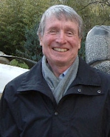
John H. Holland is best known for his role as a founding father of the complex systems approach. In particular, he developed genetic algorithms and learning classifier systems.
These foundational building blocks of an evolutionary optimization approach are now included in all texts on optimization and programming.
The naming convention used to refer to the LCS algorithm also changed since its infancy. Holland initially called it a classifier system, abbreviated either as (CS) or (CFS) [47]. From that time, it was also referred to as adaptive agents [48], cognitive systems [48] [2] and genetic-based machine learning [22] [49]. The current name of LCS was not adopted until the late 80s [50] after extending the architecture with a credit assignment component [46] [51].
This section provides a synopsis of crucial LCS concepts alongside the most popular variants and their contributions to the field.
Selected topics of LCS
Rules and Classifiers
LCS utilizes rules as a fundamental block of modelling knowledge in a general form. It comprises a condition (i.e. specified feature states) and an action (also referred to as the class). They can be interpreted using the “IF condition THEN action” logical expression. The generalization property using the “do not care” symbol # is possible when the condition part is expressed with either boolean or nominal representation. Two input situations are considered equivalent for a given classifier if the specified (non-#) values in the condition match the corresponding attributes of the two situations.
In addition to condition and action, a rule typically has many algorithm-related parameter values associated with it (like its performance or expected reward). The term classifier is used to describe a rule and its associated parameters.
It is essential to realize that LCS comprise a population of single rules that collaboratively seek to cover the problem space. The number of classifiers needed to solve the particular problem depends on factors like the problem complexity or rule representation used.
Driving Mechanisms
There are two fundamental components behind every LCS algorithm - discovery and learning (credit assignment). Both of them have generated respective fields of study, but in the context of LCS, we wish to understand their function and purpose.
Discovery component
The discovery component is responsible for exploring the search space of the target problem to uncover new rules. A vast majority of LCS algorithms employ some form of evolutionary computation, most often a genetic algorithm (GA), employing the Neo-Darwinist theory of natural selection [52] [49]. The evolution of rules is modelled after the evolution of organisms using the following biological analogies:
a code is used to represent the genotype/genome (condition),
a solution (phenotype) representation is associated with that genome (action),
a phenotype selection process (survival of the fittest) - the fittest organism (rule) has the greatest chances of reproducing and passing parts of its genome to offspring,
certain genetic genome operators are utilized in order to chase after fitter organisms (rules) [53] [54].
Two genetic operators are typically used to alter genome (rule) - mutation and crossover (recombination). The first one randomly modifies an element in an individual’s genotype (rule), while the latter recombine parts of two favourable genotypes (rules), creating a new one. The selection pressure driving better organisms (rules) to reproduce more frequently depends on the fitness function. The fitness function quantifies the optimality of a given rule, allowing it to be ranked across the entire population.
GA implementation varies in particular LCS, but the overall scheme involves evaluating all available rules, selecting the most promising offsprings (according to fitness value), applying genetic operators, introducing new offspring back to the population set and finally removing surplus or under-performing individuals.
Learning component
As mentioned, each classifier is accompanied by specific parameter values. The iterative update of them drives the process of LCS reinforcement by distributing any incoming reward signal to the classifiers that are accountable for it. This process serves two purposes:
identification of classifiers responsible for obtaining large future rewards,
encourage the discoverability of new rules (by directly affecting the fitness value).
The learning strategy depends on the nature of the problem and is realized differently in LCS implementations. In all cases, however, the process is conducted through trial-and-error interactions with the environment, where the occasional immediate reward is used to generate the policy (state-action mapping of agent-environment interactions), maximizing long-term reward [55] [56] [57].
Functional cycle
The agent interacts with the environment in consecutive trials. Each trial consists of sequential steps usually executed as follows:
Filter population \([P]\) and select classifiers where condition matches environmental perception forming a match-set \([M]\).
Determine the action that will be executed (depending on the strategy).
Narrow down the match-set by selecting only classifiers advocating proposed action - create the action-set \([A]\).
Execute the action in the environment, obtaining a new state
Refine classifiers by executing discovery and learning components.
The action selection and classifiers evolution phases are implemented individually in different LCS, but the main objective of reaching the ideal generalization level is crucial to all of them. The system should find a population that covers the search space as compactly as possible without being detrimental to the optimality of behaviour.
Pittsburgh vs Michigan approach
One of the most fundamental distinctions in LSC research is storing knowledge by using two different approaches - Michigan-style or Pittsburgh-style. The first ones were proposed by Holland [2] while the latter one by Kenneth DeJong and his student [58] [59].
The fundamental discrepancy is the structure of an individual. In Michigan systems, each individual is a classifier; in Pittsburgh, each individual is a set of classifiers - see Figure 2.1.
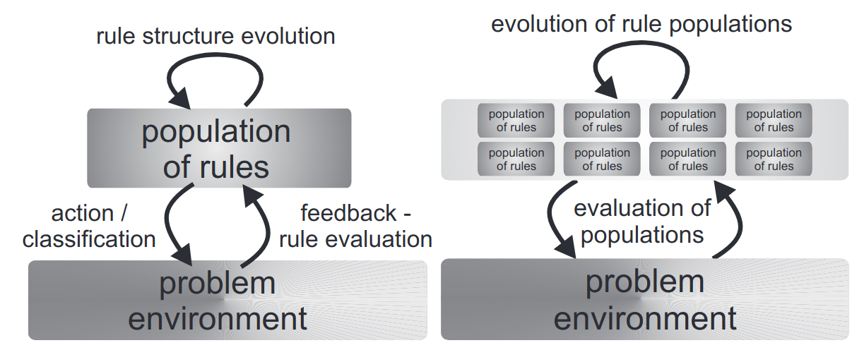
Fig. 2.1 Differences between representing knowledge in both Michigan-style and Pittsburgh-style LCS. Figure taken from [60].
Thus, the classifiers in Michigan-style LCS are being continuously evaluated and evolved, while in Pittsburgh-style LCS, the same process is much more complicated because the whole population needs to be assessed. Therefore, Michigan-style systems are typically applied in interactive, online learning problems, while Pittsburgh ones are rather suitable for offline learning [60].
This work focuses solely on the first class of LCS.
Representative LCS
This section describes Michigan-style LCS implementations contributing primarily to the current advancements.
CS-1
Two years after presenting the theoretical model of CS, Holland and Reitman proposed its implementation of CS-1 [2]. The system realized the Darwinian principle of the survival of the fittest [61] [62] and was generating adaptive behaviour by maximizing reinforcement using the bucket brigade algorithm (BBA) [61] [62].
Some internal mechanisms like the usage of an internal message list (handling all input and output communications between the system and the environment and providing a makeshift memory) or interactions between evolving both single classifier and entire population were considered difficult [63] [49]. Moreover, the obtained results were inconsistent, signifying the need for improvements.
Steward Wilson
Steward Wilson is an Independent Researcher in classifier systems and evolutionary computation.
His PhD thesis investigated what would happen if a child could ask questions and receive excellent spoken answers from a machine that connected him to recordings made by a scientist such as Carl Sagan. The results showed long, thoughtful lines of inquiry for this student-driven learning style.
ZCS
The Zeroth Level Classifier (ZCS) introduced by Wilson in 1994 [64] encompasses all LCS components while simplifying the CS-1, increasing its understandability and performance. The significant change was the removal of the internal message list (determining the rule’s format entirely by the system interface) alongside with rule-bidding credit assignment (replacing it with BBA/Q-learning algorithm [65]).
Moreover, the classifier fitness was based on the accumulated reward that the agent can get from firing the classifier, giving rise to the “strength-based” family of LCS. As a result, the discovery component eliminates classifiers providing less reward than others from the population.
ZCS achieved similar performance to CS-1, demonstrating that Holland’s idea could work even in a straightforward framework. However, the premature converge onto suboptimal rules before search space can be explored appropriately and a stable population formed led Wilson to consider other ways to achieve this.
XCS
In 1995 Wilson introduce yet another, groundbreaking modification called the eXtended Classifier System (XCS) [30] [66] [67] [68] noted for being able to reach optimal performance while evolving accurate and maximally general classifiers.
The essential changes include:
rule fitness is based on the accuracy of predictions (forming the accuracy-based LCS family),
replacement of panmictically acting GA with a niche-GA [69] (applied only in action set \([A]\) instead of globally \([P]\)),
explicit generalization mechanism (subsumption),
an adaptation of Q-Learning credit assignment.
The XCS design drives it to form an all-inclusive and accurate representation of the problem space rather than focusing on higher payoff niches. Auspicious performance results showed that RL [53] and LCS are not only linked but inherently overlapping, redefining LCSs as RL endowed with generalization capabilities [70] [71]. As a result, it becomes the most popular LCS implementation, guiding other system implementations heavily inspired by its architecture.
Modern LCS
The latest LCS advancements focus mainly on problems related to:
Knowledge visualization and rules compaction [72], [73] - new visualization techniques, termed as Feature Importance Map, Action-based Feature Importance Map and Action-based Feature’s Average value Map successfully produce human-discernable results for the investigated complex Boolean problems. Domains, where the pattern consists of 6435 different cooperating rules, were translated into concise graphs, facilitating tracking the overall training progress.
Learning with incremental data [74] [75] - a solution for extracting knowledge and utilizing it in further experiments using various deep convolutional blocks. The proposed method obtained better accuracy than other state-of-the-art algorithms using the investigated image datasets.
Classifying images using convolutional autoencoders [76] [75] [77] - high-dimensional problems are investigated by an ensemble of LCS with deep-learning methods. The input is compressed using the autoencoder and later processed by the LCS algorithm. Promising applications involve designing an intrusion detection system [78] or classifying MNIST images [37].
Dealing with perceptual aliasing environments [79] by utilizing a feature of vertebrate intelligence allowing multiple simultaneous representations of an environment at different levels of abstraction. Considering states at a constituent level enables the system to place them appropriately in holistic-level policies for multistep problems.
Anticipatory Learning Classifier Systems
The field of cognitive psychology initially guided the investigation about the presence and importance of anticipations. It was proved that “higher” animals form and exploit anticipations while adopting their behaviour in distinct tasks. Wilson noted that when simulating adaptive behaviour, the animats should be endowed with anticipations [80]. In traditional RL, the first approaches manifested in Dyna architecture [55], but due to the lack of generalization capabilities, its utilization was limited. The Anticipatory Learning Classifier Systems (ALCS) aims to bridge the gap for exploiting the generalization capabilities while including the explicit notion of anticipations.
CFCS2
Riolo laid the foundations towards including predictions in 1991 by introducing a modification called CFCS2 [81]. It addressed the task of performing “latent learning” or “lookahead planning” where “actions are based on predictions of future states of the world, using both current information and past experience as embodied in the agent’s internal models of the world” [82].
CFCS2 used “tags” to specify if a current action posted to a message list refers to actual action or anticipation, claiming a reduction in the learning time for general sequential decision tasks. Riolo was able to show the possibilities of latent learning and lookahead planning, but the implicit formation of anticipations appeared to be misleading. Additionally, the CFCS2 did not achieve any generalization capabilities.
ACS
The first system competent of evolving a maximally generalized, accurate and complete mapping of all possible situation-effect-action triples observable in the environment - the Anticipatory Classifier System (ACS) was introduced by Stolzmann in 1997 [83] [84].
The rule structure was enhanced with an anticipatory or effect part that explicitly anticipates the effects of an action in a given situation. The effect part could determine which attributes change after executing an action by using a “pass-through” symbol - \(\#\), which significantly enhances the rule’s interpretability. In order to perform latent learning, forming and refining classifiers, a discovery component - the Anticipatory Learning Process (ALP) was introduced.
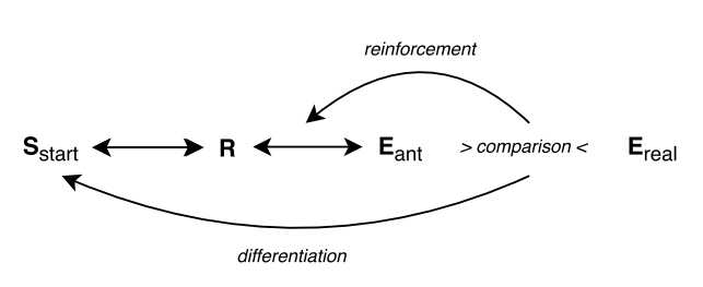
ALP realizes the psychological Hoffmann’s anticipatory behavioral control theory [85] [86] stating that conditional action-effects relations are learned latently using anticipations, which he further refined in [87]. The following points (visualised in Figure 2.2) can be distinguished:
Any behavioural act or response (\(R\)) is accompanied by anticipation of its effects.
The anticipations of the effects \(E_{ant}\) are compared with the real effects \(E_{real}\).
When the anticipations are correct, the bond between response and anticipation is strengthened and weakened otherwise.
Behavioural stimuli further differentiate the \(R-E_{ant}\) relations.
The implementation of this component compares the obtained state \(\sigma_{t+1}\) with the classifier’s anticipation \(\sigma_{t+1}^{ant}\). Then, the quality parameter of the involved classifier is updated according to four possible scenarios:
Useless case. After performing an action, no change in perception is perceived from the environment. The classifier’s quality decreases.
Expected case. When the newly observed state matches the classifier prediction. Classifiers’ quality is increased.
Correctable case. When new state \(\sigma(t+1)\) does not match the anticipation of \(cl.E\). A new classifier with a matching effect part is generated.
Not correctable case. When new state \(\sigma(t+1)\) does not match the anticipation of \(\sigma_{t+1}^{ant}\), and it is not possible to correct the classifier, then its quality is penalized like in the useless case.
The classifiers are removed from the population if they became inadequate - the quality metrics fall below a threshold denoted by the \(\theta_i\) parameter.
The proposed architecture was capable of solving multistep problems, planning, speeding up learning or disambiguating perceptual aliasing.
import lcs.agents.acs2 as acs2
from lcs.metrics import population_metrics

from typing import Optional, Tuple

def maze_metrics(agent, env):
    metrics = {}
    metrics.update(population_metrics(agent.population, env))
    return metrics

acs2_base_params = {
    'classifier_length': 8,
    'number_of_possible_actions': 8,
    'biased_exploration': 0,
    'metrics_trial_frequency': 1,
    'user_metrics_collector_fcn': maze_metrics
}

def run_acs2_explore_exploit(env, explore_trials, exploit_trials, **config):
    cfg = acs2.Configuration(**config)

    # explore phase
    agent = acs2.ACS2(cfg)
    metrics_explore = agent.explore(env, explore_trials)

    # exploit phase
    agent_exploit = acs2.ACS2(cfg, copy(agent.population))
    metrics_exploit = agent_exploit.exploit(env, exploit_trials)

    return (agent, metrics_explore), (agent_exploit, metrics_exploit)

def find_best_classifier(population: acs2.ClassifiersList, situation: Perception) -> Optional[acs2.Classifier]:
    match_set = population.form_match_set(situation)
    anticipated_change_cls = [cl for cl in match_set if cl.does_anticipate_change()]

    if len(anticipated_change_cls) > 0:
        return max(anticipated_change_cls, key=lambda cl: cl.fitness)

    return None

def build_fitness_and_action_matrices(env, population) -> Tuple:
    original = env.env.maze.matrix

    fitness = original.copy()
    action = original.copy().astype(str)

    action_lookup = {
        0: u'↑', 1: u'↗', 2: u'→', 3: u'↘',
        4: u'↓', 5: u'↙', 6: u'←', 7: u'↖'
    }

    for index, x in np.ndenumerate(original):
        if x == 0:  # path
            perception = env.env.maze.perception(index)
            best_cl = find_best_classifier(population, perception)

            if best_cl:
                fitness[index] = best_cl.fitness
                action[index] = action_lookup[best_cl.action]
            else:
                fitness[index] = -1
                action[index] = '?'

        if x == 1:  # wall
            fitness[index] = 0
            action[index] = '\#'

        if x == 9:  # reward
            # add 500 to make it more distinguishable
            fitness[index] = fitness.max() + 500
            action[index] = 'R'

    return fitness, action

def plot_policy(env, fitness_matrix, action_matrix, plot_filename=None):
    fig, ax = plt.subplots(1, 1, figsize=(14, 8))

    max_x, max_y = env.env.maze.matrix.shape

    # Render maze as image
    plt.imshow(fitness_matrix, interpolation='nearest', cmap='Reds', aspect='auto', extent=[0, max_x, max_y, 0])

    # Add labels to each cell
    for (y, x), val in np.ndenumerate(action_matrix):
        plt.text(x + 0.4, y + 0.5, "${}$".format(val))

    ax.set_title("ACS2 policy in Maze5 environment", fontsize=24)
    ax.set_xlabel('x', fontsize=18)
    ax.set_ylabel('y', fontsize=18)
    ax.set_xlim(0, max_x)
    ax.set_ylim(max_y, 0)
    ax.set_xticks(range(0, max_x))
    ax.set_yticks(range(0, max_y))
    ax.grid(True)

    if plot_filename:
        fig.savefig(plot_filename, dpi=PLOT_DPI)

    return fig

@get_from_cache_or_run(cache_path=f'{cache_dir}/acs2_maze5.dill')
def run_acs2_in_maze5():
    env = gym.make('Maze5-v0')
    explore_phase, exploit_phase = run_acs2_explore_exploit(env, explore_trials=5000, exploit_trials=100, **acs2_base_params)
    return env, explore_phase, exploit_phase

# Run computation
env_, explore_, exploit_ = run_acs2_in_maze5()

# Plot the policy
fitness_matrix, action_matrix = build_fitness_and_action_matrices(env_, explore_[0].population)
acs2_policy_fig = plot_policy(env_, fitness_matrix, action_matrix, plot_filename=f'{plot_dir}/acs2-maze5-policy.png')

glue('acs2_policy_fig', acs2_policy_fig, display=False)
glue('acs2_population_size', len(explore_[0].population), display=False)
ACS2
Later, in 2002 Martin Butz [26] [88] extended ACS by introducing a system named ACS2. The significant changes from the previous version include:
application of learning component across the whole action set \([A]\) (all classifiers from \([M]\) advocating selected action),
introduction of GA component,
refinement of learning component utilizing the Q-learning [55] algorithm,
condition-action-effect triples that anticipate no change in the environment are explicitly encompassed in population,
add mark property to classifier, recording the properties in which it did not perform correctly before.
The ALP process was refined due to its delicate nature. The first improvement relates to the process of improving new classifier generation by covering all possible condition-action-effect triples. The process called COVERING is called when there is no classifier in the action set \([A]\) representing the encountered situation. A newly created classifier specifies all changes from the previous situation \(\sigma_{t-1}\) to situation \(\sigma\) in condition and effect part. Second, because the offspring might be introduced by ALP and GA, the insertion process must be cautious. A subsumption operation checks if one classifier is not covered by the other, more general one. For a classifier \(cl_{sub}\) to subsume another classifier \(cl_{tos}\), the subsumer needs to be experienced, reliable and not marked. Moreover, the subsumer’s condition part needs to be syntactically more general, and the effect part needs to be identical.
The GA algorithm is responsible for generalizing the condition parts. The method starts by determining if the GA should actually take place, controlled by the \(t_{ga}\) time stamp and the actual time \(t\). If a GA takes place, preferable accurate, over-specified classifiers are selected, mutated and crossed, see [88] for a detailed explanation.
Experiments showed that the genetic generalization process in ACS2 decreased the population size and consequently speed up the computational process.
Figure 2.3 demonstrates an example of RL policy generated by a population of 322 classifiers trained over 5000 trials operating in popular Maze5 benchmarking problem. The model knows the consequences of each available action in every possible state; therefore, estimating the fitness value of each classifier can suggest the most promising action. The learning can be still optimized by using cognitive mechanisms like lookahead planning [82].
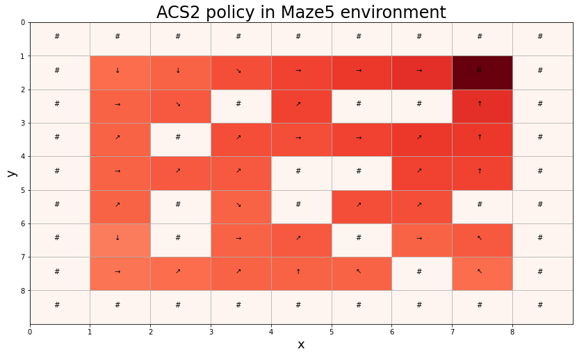
Fig. 2.3 Policy generated by ACS2 in Maze5 environment. The saturation of the red colour reflects the best classifier fitness value. The agent is inserted randomly on the red field in each trial to reach the reward state “R” by executing one of the eight possible actions.
The recent advancements include the integration of the action planning mechanism [89], PEPACS extension where the concept of Probability-Enhanced-Predictions is used for handling non-deterministic environments [90] or BACS tackling the issue of perceptual aliasing by building Behavioral Sequences [91].
YACS
In the same year, 2002, Gérard introduced a “Yet Another Classifier System” (YACS) [92]. It shares the same C-A-E classifier structure as ACS and ACS2, but the essential conceptual difference is that YACS is designed to decorrelate the acquisition of relevant \(C\) and \(E\) parts by building them independently using a set of heuristics. The latent learning process is designed to set the E parts to perceived changes in the environment and then discover relevant C parts. Moreover, it does not take advantage of genetic generalization mechanisms relying on the discovery process to determine significant attributes correctly. In order to compute the optimal policy YACS memorizes internally every encountered state and uses a simplified variety of value iteration algorithm.
The evaluation was performed only in simple multistep maze environments reaching near optimal solutions. The specialization process in YACS leads to less over-specialization than the corresponding process in ACS but still suffers from the lack of a dedicated generalization mechanism. Additionally, the YACS cannot deal with uncertainty and operate only in Markov and deterministic environments.
import lcs.agents.macs.macs as macs

maze228_env = gym.make('Maze228-v0')

def _calculate_rotating_maze_knowledge(agent: macs.MACS, env):
    transitions = env.env.transitions
    covered_transitions = 0

    for p0, a, p1 in transitions:
        p0p = Perception(list(map(str, p0)))
        p1p = Perception(list(map(str, p1)))
        anticipations = list(agent.get_anticipations(p0p, a))

        # accurate classifiers
        if len(anticipations) == 1 and anticipations[0] == p1p:
            covered_transitions += 1

    return covered_transitions / len(transitions)

def _macs_metrics(agent: macs.MACS, env):
    population = agent.population
    return {
        'pop': len(population),
        'situations': len(agent.desirability_values),
        '0_cls': len([cl for cl in population if cl.action == 0 and cl.is_accurate]),
        '1_cls': len([cl for cl in population if cl.action == 1 and cl.is_accurate]),
        '2_cls': len([cl for cl in population if cl.action == 2 and cl.is_accurate]),
        'knowledge': _calculate_rotating_maze_knowledge(agent, env)
    }

@get_from_cache_or_run(cache_path=f'{cache_dir}/macs_maze228.dill')
def run_macs_in_maze228(env):
    cfg = macs.Configuration(classifier_length=9,
                        number_of_possible_actions=3,
                        feature_possible_values=[{'0', '1', '9'}] * 8 + [{'0', '9'}],
                        estimate_expected_improvements=True,
                        metrics_trial_frequency=10,
                        user_metrics_collector_fcn=_macs_metrics)

    agent = macs.MACS(cfg)
    metrics = agent.explore(env, 100)

    return agent, metrics

# run computations
macs_agent, macs_metrics = run_macs_in_maze228(maze228_env)

# visualization
random.seed(129)  # found experimentally
maze228_env.reset()
left_from_reward = maze228_env.env.maze.perception()

glue('maze228_perception', "".join(left_from_reward), display=False)
glue('macs_maze228_population', len(macs_agent.population), display=False)
MACS
Knowing certain limitations of ACS and YACS in 2005, Gérard proposed a Modular Anticipatory Classifier System (MACS) [93]. He realised that specific problems would be better approached with a different representation of the rule formalism. While in ACS and YACS, generalisation and selective attention are afforded by the joint use of don’t care and pass-through symbols, it can detect if a particular attribute is changing or not. The efficient representation of regularities across different attributes is impossible because each situation is considered an unsecable whole.
The particularity of such regularity is that the new value of an attribute depends on the previous value of another one. To overcome this problem, the pass-through symbol (#) in the expected situation \(E\) was replaced with the don’t know symbol (?). This formalism allows decorrelating the attributes from \(E\), where previously, the new value of an attribute may only depend upon the previous value of the same attribute.
This modification resulted in specific rule representation and modified architecture for latent learning. Each time a match-set \([M]\) is built a rule for each attribute change is picked, and then the final anticipation is combined.
The example of differences between rules is illustrated using the Maze228 problem [93]. The agent’s goal is to obtain the final reward. It perceives its surroundings (wall - 1, path - 0 or reward - 9) using the clockwise vector of nine attributes and can execute three actions - step ahead - 0, rotate left - 1 or rotate right - 2. Assume that the current situation is depicted on the plot below, where the agent is located on the left of the reward, and its actual perception is '009111000'.
maze228_env.render()
■ ■ ■ ■ ■ ■ ■
■ □ ■ □ ■ □ ■
■ □ □ □ □ □ ■
■ □ ■ ■ □ □ ■
■ □ ■ □ □ □ ■
■ □ □ □ A $ ■
■ ■ ■ ■ ■ ■ ■
After training, MACS represents complete knowledge about this environment using 211 classifiers. The final anticipation is obtained after combining particular classifiers selected for each action. This process for the examined environmental state is shown in the table below.
s = sorted(macs_agent.population.form_match_set(left_from_reward), key=lambda cl: cl.action)
macs_knowledge = {}

for action, group_cl in groupby(s, key=lambda cl: cl.action):
    macs_knowledge[action] = {}
    macs_knowledge[action]['anticipation'] = f'<code>{"".join([p for p in macs_agent.get_anticipations(left_from_reward, action)][0])}</code>'
    macs_knowledge[action]['classifiers'] = []

    for cl in sorted(group_cl, key=lambda cl: cl.effect):
        macs_knowledge[action]['classifiers'].append(f'<code>{cl.condition} {cl.action} {cl.effect}</code>')

# prepare table
macs_table_data = [
    ['<b>classifiers</b>', '<br/>'.join(macs_knowledge[0]['classifiers']), '<br/>'.join(macs_knowledge[1]['classifiers']), '<br/>'.join(macs_knowledge[2]['classifiers'])],
    ['<b>anticipation</b>', macs_knowledge[0]['anticipation'], macs_knowledge[1]['anticipation'], macs_knowledge[2]['anticipation']],
]

macs_table = tabulate(macs_table_data, headers=['Step ahead', 'Rotate left', 'Rotate right'], tablefmt="unsafehtml", stralign='right')
display(HTML(macs_table))
| Step ahead | Rotate left | Rotate right | |
|---|---|---|---|
| classifiers | 0#9###### 0 0????????#0###10## 0 ?0???????0#9##1### 0 ?0???????#0####### 0 ??0??????0#9###### 0 ???9?????0######## 0 ????0????0#####0## 0 ?????0???#######0# 0 ??????0??##9###### 0 ??????0??##91#10## 0 ???????1?0######## 0 ????????0 | ######0## 1 0????????#######0# 1 ?0???????0######## 1 ??0??????#0####### 1 ???0?????##9###### 1 ????9????###1##### 1 ?????1???####1#### 1 ??????1??#####1### 1 ???????1?######### 1 ????????0 | ##9###### 2 9????????###1##### 2 ?1???????####1#### 2 ??1??????#####1### 2 ???1?????######0## 2 ????0????#######0# 2 ?????0???0######## 2 ??????0??#0####### 2 ???????0?######### 2 ????????0 |
| anticipation | 000900010 | 000091110 | 911100000 |
def _acs2_metrics(agent: acs2.ACS2, env):
    population = agent.population
    reliable = [cl for cl in population if cl.is_reliable()]
    return {
        'pop': len(population),
        'rel': len(reliable)
    }

@get_from_cache_or_run(cache_path=f'{cache_dir}/acs2_maze228.dill')
def run_acs2_in_maze228(env):
    cfg = acs2.Configuration(classifier_length=9,
                        number_of_possible_actions=3,
                        metrics_trial_frequency=1,
                        user_metrics_collector_fcn=_acs2_metrics,
                        do_ga=False)

    agent = acs2.ACS2(cfg)
    metrics = agent.explore(env, 5000)

    return agent, metrics

acs2_agent, acs2_metrics = run_acs2_in_maze228(maze228_env)

reliable_classifiers = [cl for cl in acs2_agent.population if cl.is_reliable()]

glue('acs2_maze228_population', len(reliable_classifiers), display=False)
On the other side, the ACS2 creates a much larger population of 402 reliable classifiers. There is a single classifier describing the change of multiple attributes for each action. The anticipation in both cases is the same, but due to the specific nature of this problem, MACS results in an overall more compact internal model of the environment.
acs2_knowledge = {}

for cl in acs2_agent.population.form_match_set(left_from_reward):
    acs2_knowledge[cl.action] = {}
    acs2_knowledge[cl.action]['classifiers'] = []
    acs2_knowledge[cl.action]['anticipation'] = f'<code>{"".join(cl.get_best_anticipation(left_from_reward))}</code>'

    if cl.is_reliable():
        acs2_knowledge[cl.action]['classifiers'].append(f'<code>{cl.condition} {cl.action} {cl.effect}</code>')


# prepare table
acs2_table_data = [
    ['<b>classifiers</b>', '<br/>'.join(acs2_knowledge[0]['classifiers']), '<br/>'.join(acs2_knowledge[1]['classifiers']), '<br/>'.join(acs2_knowledge[2]['classifiers'])],
    ['<b>anticipation</b>', acs2_knowledge[0]['anticipation'], acs2_knowledge[1]['anticipation'], acs2_knowledge[2]['anticipation']],
]

acs2_table = tabulate(acs2_table_data, headers=['Step ahead', 'Rotate left', 'Rotate right'], tablefmt="unsafehtml", stralign='right')
display(HTML(acs2_table))
| Step ahead | Rotate left | Rotate right | |
|---|---|---|---|
| classifiers | ##9111#0# 0 ##0900#1# | ##911#00# 1 ##009#11# | 009#11### 2 911#00### |
| anticipation | 000900010 | 000091110 | 911100000 |