2.4. Statistical verification of results¶

In order to assess the significance and performance of obtained results, two statistical approaches were used. The majority of metrics were compared using the Bayesian estimation (BEST) method [114], while the other straightforward metrics were just averaged.

Bayesian analysis¶

The Bayesian approach towards comparing data from multiple groups was used instead of traditional methods of null hypothesis significance testing (NHST). They are more intuitive than the calculation and interpretation of p-value scores, provides complete information about credible parameter values and allow more coherent inferences from data [115].

Benavoli depicted the perils of the frequentist NHST approach when comparing machine learning classifiers in [116], which is particularly suited for this work. He points out the following reasons against using the NHST methods:

it does not estimate the probability of hypotheses,
point-wise null hypotheses are practically always false,
the p-value does not separate between the effect size and the sample size,
it ignores magnitude and uncertainty,
it yields no information about the null hypothesis,
there is no principled way to decide the \(\alpha\) level.

Additionally, in 2016 the American Statistical Association made a statement against p-values [117] which might be a motivation for other disciplines to pursue the Bayesian approach.

In this work, we focus on establishing a descriptive mathematical model of the data \(D\) using the Bayes’ theorem deriving the posterior probability as a consequence of two antecedents: a prior probability and a “likelihood function” derived from a statistical model for the observed data (2.6).

(2.6)¶\[\underbrace{p(\mu, \sigma, \nu|D)}_{\text{posterior}} = \underbrace{p(D|\mu, \sigma, \nu)}_{\text{likelihood}} \times \underbrace{p(\mu, \sigma, \nu)}_{\text{prior}} \big/ \underbrace{p(D)}_{\text{evidence}}\]

Each experiment is performed 50 times, generating independent samples, which according to the Central Limit Theorem, should be enough to consider it is approximating the normal distribution [118] [119]. To further provide a robust solution towards dealing with potential outliers, the Student t-distribution is chosen. The prior distribution, described with three parameters - \(\mu\) (expected mean value), \(\sigma\) (standard deviation) and \(\nu\) (degrees of freedom) is presented using the Equation (2.7). The standard deviation \(\sigma\) parameter uniformly covers a vast possible parameter space. The degrees of freedom follows a shifted exponential distribution controlling the normality of the data. When \(\nu>30\), the Student-t distribution is close to a normal distribution. However, if \(\nu\) is small, Student t-distributions have a heavy tail. Therefore, value of \(\nu \sim \mathrm{Exp}(\frac{1}{29})\) allows the model to be more tolerant for potential outliers.

(2.7)¶\[\begin{split}\begin{align} \mu &\sim \mathrm{N}(\mu_D, \sigma^2_D) \\ \sigma &\sim \mathrm{U}(\frac{1}{100}, 1000) \\ \nu &\sim \mathrm{Exp}(\frac{1}{29}) \end{align}\end{split}\]

The posterior distribution is approximated arbitrarily high accuracy by generating a large representative sample using Markov chain Monte Carlo (MCMC) methods. Its sample provides thousands of combinations of parameter values \(<\mu, \sigma, \nu>\). Each such combination of values is representative of credible parameter values that simultaneously accommodate the observed data and the prior distribution. From the MCMC sample, one can infer credible parameter values like the mean or standard deviation.

Example¶

To show an example of this technique, the performance of an ACS2 algorithm operating in a multistep, toy-problem - Simple Maze environment [120] (see Figure 2.7) will be discussed using three methods - the summary statistics, frequentist approach and the Bayesian estimation.

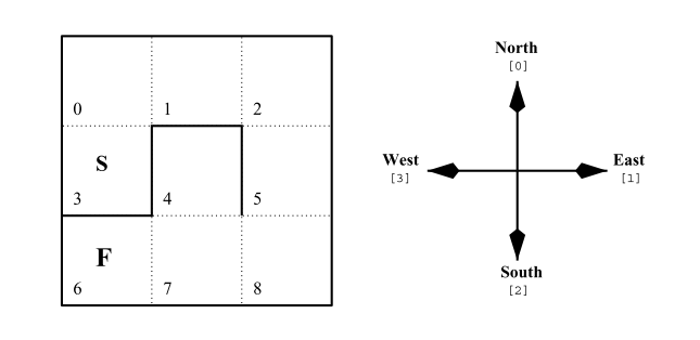
Fig. 2.7 The Simple Maze environment is a Partially Observable Markov Decision Problem where the agent is placed in the starting location (denoted as “S”), at the beginning of each new trial, and the goal is to reach the final state “F” by executing four possible actions – moving north, east, south or west. The bolded lines represent the walls, and the goal can be reached optimally in seven successive steps.¶

import gym
import lcs.agents.acs2 as acs2

SIMPLE_MAZE_TRIALS = 500
LEARNING_RATE = 0.1
DISCOUNT_FACTOR = 0.8


def simple_maze_env_provider():
    import gym_yacs_simple_maze  # noqa: F401
    return gym.make('SimpleMaze-v0')


def custom_metrics(agent, env):
    population = agent.population
    return {
        'pop': len(population),
        'reliable': len([cl for cl in population if cl.is_reliable()])
    }


@get_from_cache_or_run(cache_path=f'{cache_dir}/simple-maze/acs2.dill')
@repeat(num_times=NUM_EXPERIMENTS, use_ray=True)
def run_acs2(env_provider):
    simple_maze_env = env_provider()

    cfg = acs2.Configuration(
        classifier_length=4,
        number_of_possible_actions=4,
        beta=LEARNING_RATE,
        gamma=DISCOUNT_FACTOR,
        do_ga=False,
        metrics_trial_frequency=1,
        user_metrics_collector_fcn=custom_metrics)

    agent = acs2.ACS2(cfg)
    return agent.explore(simple_maze_env, SIMPLE_MAZE_TRIALS)


@get_from_cache_or_run(cache_path=f'{cache_dir}/simple-maze/acs2ga.dill')
@repeat(num_times=NUM_EXPERIMENTS, use_ray=True)
def run_acs2ga(env_provider):
    simple_maze_env = env_provider()

    cfg = acs2.Configuration(
        classifier_length=4,
        number_of_possible_actions=4,
        beta=LEARNING_RATE,
        gamma=DISCOUNT_FACTOR,
        do_ga=True,
        metrics_trial_frequency=1,
        user_metrics_collector_fcn=custom_metrics)

    agent = acs2.ACS2(cfg)
    return agent.explore(simple_maze_env, SIMPLE_MAZE_TRIALS)


# run computations
acs2_runs_metrics = run_acs2(simple_maze_env_provider)
acs2ga_runs_metrics = run_acs2ga(simple_maze_env_provider)

# build dataframes
acs2_metrics_df = pd.DataFrame(itertools.chain(*acs2_runs_metrics))
acs2ga_metrics_df = pd.DataFrame(itertools.chain(*acs2ga_runs_metrics))

# extract population size in last trial
acs2_population_counts = acs2_metrics_df.query(f'trial == {SIMPLE_MAZE_TRIALS - 1}')['reliable']
acs2ga_population_counts = acs2ga_metrics_df.query(f'trial == {SIMPLE_MAZE_TRIALS - 1}')['reliable']

# glue variables
glue('stats_simple_maze_trials', SIMPLE_MAZE_TRIALS, display=False)

The ACS2 agent will be tested in two variants - with and without the genetic algorithm modification. All other settings are identical. Both agents in each experiment will execute 500 trials, each time randomly selecting an action. Finally, each such experiment will be independently repeated 50 times.

Null hypothesis

The classifier population sizes obtained by ACS2 and ACS2 GA in the last trial \(x\) are equal.

Descriptive statistics

The first option is to understand the data and extract basic summary statistics. Figure 2.8 presents a whisker plot showing basic data aggregations like the minimum, first quartile, median, third quartile, maximum values alongside the histogram visualization. While the values look similar, it is still unclear whether they can be considered the same.

def plot_summary_statistics(data, labels, plot_filename=None):
    fig = plt.figure(figsize=(14, 8))
    colors = ['lightblue', 'lightgreen']

    # boxplot
    ax1 = fig.add_subplot(121)

    bp = ax1.boxplot(data,
                     patch_artist=True,
                     labels=labels)

    for patch, color in zip(bp['boxes'], colors):
        patch.set_facecolor(color)

    ax1.set_title('Whisker plot', pad=20)
    ax1.set_ylabel('Observed population size values')
    ax1.grid(which='major', axis='y', linestyle='--')

    # histogram
    ax2 = fig.add_subplot(122)
    for d, l, c in zip(data, labels, colors):
        ax2.hist(d, bins=10, label=l, color=c, edgecolor='black', alpha=.8, linewidth=1)

    ax2.set_title('Histogram', pad=20)
    ax2.grid(which='major', axis='y', linestyle='--')
    ax2.legend()

    # common settings
    fig.suptitle('ACS2 and ACS2 GA Comparison', fontweight='bold')
    fig.subplots_adjust(top=0.85)

    if plot_filename:
        fig.savefig(plot_filename, dpi=PLOT_DPI)

    return fig


summary_plot_fig = plot_summary_statistics(
    [acs2_population_counts.to_numpy(), acs2ga_population_counts.to_numpy()],
    ['ACS2', 'ACS2 GA'],
    plot_filename=f'{plot_dir}/summary-stats.png')

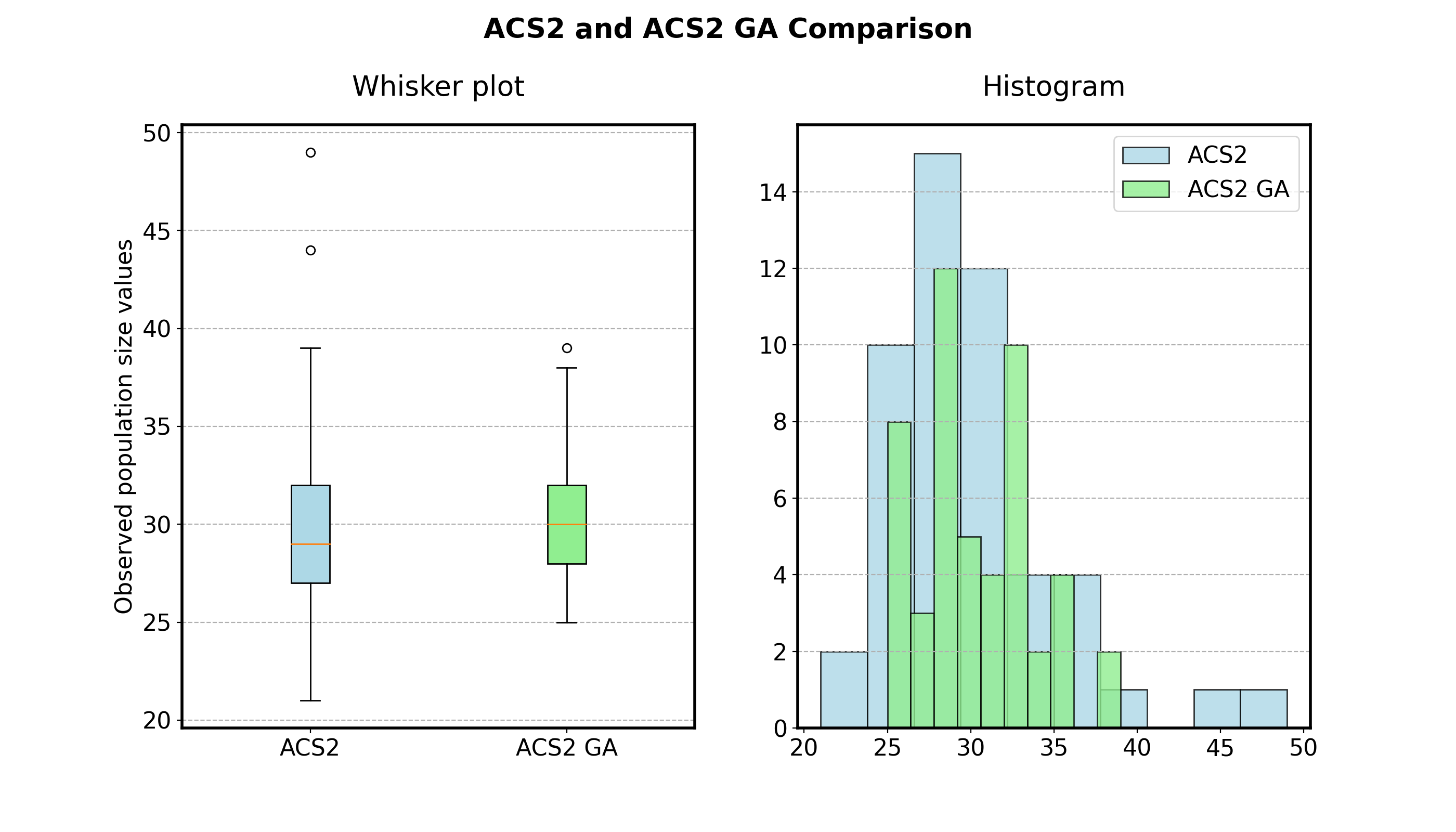
Fig. 2.8 Descriptive statistics depicting population size obtained after executing two versions of the ACS2 agent in the Simple Maze environment.¶

Frequentist approach

For the frequentist approach first two hypotheses about data distribution are formed:

\[\begin{split}\begin{align*} &H_0: \text{The classifier population sizes obtained by ACS2 and ACS2 GA are equal}\\ &H_1: \text{The classifier population sizes obtained by ACS2 and ACS2 GA are different} \end{align*}\end{split}\]

In traditional NHST workflow, the first step would be to apply normality tests to verify whether the data is normally distributed. However, looking at the histograms from the Figure 2.8 we might assume that the data follow the Gaussian distribution and skip it.

If the \(H_0\) hypothesis is rejected, there is no significant difference between the means. To do so, a p-value will be calculated and compared with a certain threshold \(\alpha \leq 0.05\). If the p-value falls below the threshold, it means that the null hypothesis \(H_0\) can be rejected and there is 95% confidence that both means are significantly different.

from scipy.stats import ttest_ind

# don't assume equal variances
value, pvalue = ttest_ind(acs2_population_counts, acs2ga_population_counts, equal_var=False)

glue('stats-pvalue', round(pvalue, 2), display=False)

In this case, after running the two-sided t-Test, the calculated p-value is 0.68, which indicates strong evidence for the \(H_0\) hypothesis, meaning that it is retained. Remember that NHST does not accept the null hypothesis; it can be only rejected or failed to be rejected. Stating that it is correct implies 100% certainty, which is not valid in this methodology.

Bayesian estimation

Throughout this work a PyMC3 open-sourced Python framework is used for the probabilistic programming. Figure 2.9 depicts two separate Student-t posterior distribution hyper-parameters estimated by using the MCMC method.

from src.bayes_estimation import bayes_estimate


@get_from_cache_or_run(cache_path=f'{cache_dir}/simple-maze/bayes-acs2.dill')
def bayes_estimate_acs2(data):
    return bayes_estimate(data)


@get_from_cache_or_run(cache_path=f'{cache_dir}/simple-maze/bayes-acs2ga.dill')
def bayes_estimate_acs2ga(data):
    return bayes_estimate(data)


# run estimations
bayes_acs2_trace = bayes_estimate_acs2(acs2_population_counts.to_numpy())
bayes_acs2ga_trace = bayes_estimate_acs2ga(acs2ga_population_counts.to_numpy())


def plot_bayes_parameters(data, labels, plot_filename=None):
    colors = ['lightblue', 'lightgreen']
    hist_kwargs = {'bins': 20, 'edgecolor': 'black', 'alpha': .8, 'linewidth': 1}

    fig, axs = plt.subplots(2, 3, figsize=(16, 8))

    for i, (d, l, c) in enumerate(zip(data, labels, colors)):
        axs[i][0].hist(d['mu'], color=c, label=l, **hist_kwargs)
        axs[i][0].set_title(f'$\mu_{{{l}}}$')

        axs[i][1].hist(d['std'], color=c, label=l, **hist_kwargs)
        axs[i][1].set_title(f'$\sigma_{{{l}}}$')

        axs[i][2].hist(d['nu'], color=c, label=l, **hist_kwargs)
        axs[i][2].set_title(fr'$\nu_{{{l}}}$')

    # share axes
    axs[0][0].sharex(axs[1][0])
    axs[0][1].sharex(axs[1][1])
    axs[0][2].sharex(axs[1][2])

    # common
    handles, labels = [(a + b) for a, b in zip(axs[0][0].get_legend_handles_labels(), axs[1][0].get_legend_handles_labels())]
    fig.suptitle('Posterior distribution of ACS2 and ACS2 GA Student-t parameters', fontweight='bold')
    fig.legend(handles, labels, loc='lower center', ncol=2, bbox_to_anchor=(0.5, -0.1))
    fig.tight_layout()

    if plot_filename:
        fig.savefig(plot_filename, dpi=PLOT_DPI)

    return fig


bayes_parameters_fig = plot_bayes_parameters(
    [bayes_acs2_trace, bayes_acs2ga_trace],
    ['ACS2', 'ACS2 GA'],
    plot_filename=f'{plot_dir}/stats-bayes-parameters.png')

glue('stats_bayes_params_fig', bayes_parameters_fig, display=False)

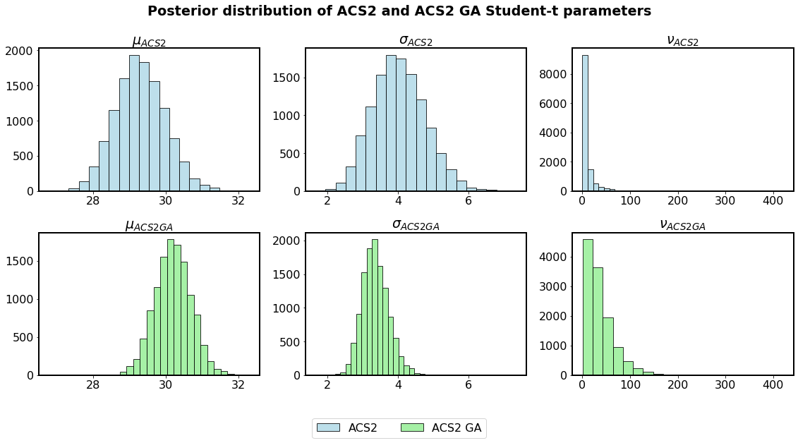
Fig. 2.9 Parameter distributions of Student-t estimation of population size data for two agents.¶

The posterior distribution allows assessing the null value more credibly. Contrary to NHST, it can also accept \(H_0\). To do so, a researcher defines a region of practical equivalence (ROPE) [121], enclosing the values of the parameter that are deemed to be negligibly different from the null values for practical purposes. When nearly all the credible values fall within the ROPE, the null value is said to be accepted for practical purposes.

Figure 2.10 shows the graphical example of verifying the null hypothesis using the difference between two posterior distributions of population means \(\mu_{ACS2}-\mu_{ACS2GA}\). The ROPE region (red sector) was assumed to be \([-1, 1]\), which means that the difference of one classifier is acceptable to consider two populations equal. Blue lines represent the area of credible values of the previously calculated difference. Since the credible value region does not fall into the ROPE region, the \(H_0\) is rejected (while the NHST approach retained it).

import arviz
import numpy as np
from scipy.stats import gaussian_kde

def plot_kde(data_diff, rope=None, hdi_prob=0.95, plot_filename=None):
    if rope is None:
        rope = [-1, 1]

    fig = plt.figure(figsize=(16, 8))
    ax = fig.add_subplot(111)

    x = np.linspace(min(data_diff), max(data_diff), 1000)
    gkde = gaussian_kde(data_diff)
    ax.plot(x, gkde(x), color='orange', label='$\mu_{ACS2}-\mu_{ACS2GA}$')
    ax.fill_between(x, gkde(x), alpha=0.1, color='orange')

    # no difference vertical line
    ax.axvline(0, color='black', alpha=0.5, linestyle='--')

    # high density interval
    hdi = arviz.hdi(data_diff, hdi_prob=0.95)
    ax.axvline(x=hdi[0], linestyle='--', color='blue', label=f'{int(hdi_prob * 100)}% HDI')
    ax.axvline(x=hdi[1], linestyle='--', color='blue')

    # ROPE
    ax.axvline(x=rope[0], linestyle='--', color='red', label='ROPE')
    ax.axvline(x=rope[1], linestyle='--', color='red')
    ax.fill_between(np.arange(rope[0], rope[1], 0.01), 0.5, color='red', alpha=0.05)

    ax.set_ylim(0, 0.5)
    fig.suptitle(r'Assessing $H_0$ using Bayes estimation', fontweight='bold')

    plt.legend()

    if plot_filename:
        fig.savefig(plot_filename, dpi=PLOT_DPI)

    return fig


data_diff = bayes_acs2_trace['mu'] - bayes_acs2ga_trace['mu']

bayes_delta_fig = plot_kde(data_diff, plot_filename=f'{plot_dir}/stats-bayes-delta.png')

glue('stats_bayes_delta_fig', bayes_delta_fig, display=False)

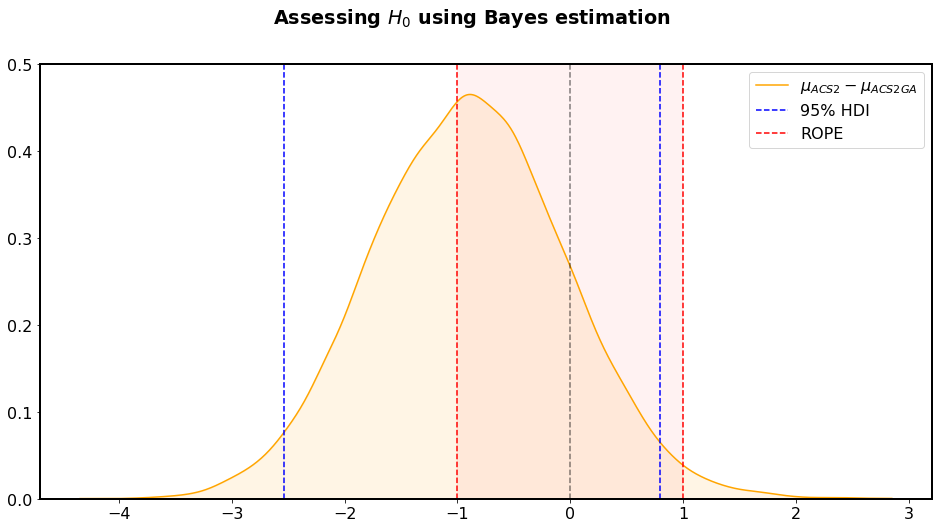
Fig. 2.10 Assessing \(H_0\) using the probabilistic density function of \(\mu\) parameter difference of two examined populations. The ROPE interval was chosen to \([-1, 1]\) meaning that a difference of one classifier can be neglected in terms of population equality. Even though the mean difference is less than one, the \(H_0\) is rejected because the HDI region is not contained within the ROPE.¶

Real-valued Anticipatory Classifier System

Statistical verification of results

Contents

2.4. Statistical verification of results¶

Bayesian analysis¶

Example¶