Experiment 1 - Straight Corridor¶

The following section describes the differences observed between using the ACS2 with standard discounted reward distribution and two proposed modifications. In all cases, the experiments were performed in an explore-exploit manner for the total number of 10000 trials, where the mode was alternating in each trial. Additionally, for better reference and benchmarking purposes, basic implementations of Q-Learning and R-Learning algorithms were also introduced and used with the same parameter settings as ACS2 and AACS2.

The most important thing was to distinguish whether the new reward distribution proposition still allows the agent to successfully update the classifier’s parameter to allow the exploitation of the environment. To illustrate this, figures presenting the number of steps to the final location, estimated average change during learning, and the reward payoff landscape across all possible state-action pairs were plotted for the Corridor of size \(n=20\) - Figure 5.2.

To assure that the modification worked as expected, the statistical inference of obtained result was performed on a scaled version of the problem. Each experiment is averaged over 50 independent runs.

def corridor20_env_provider():
    import gym_corridor  # noqa: F401
    return CorridorObservationWrapper(gym.make(f'corridor-20-v0'))

def corridor40_env_provider():
    import gym_corridor  # noqa: F401
    return CorridorObservationWrapper(gym.make(f'corridor-40-v0'))

def corridor100_env_provider():
    import gym_corridor  # noqa: F401
    return CorridorObservationWrapper(gym.make(f'corridor-100-v0'))

# Set ACS2/AACS2 configuration parameter dictionary
basic_cfg = {
    'perception_bits': 1,
    'possible_actions': 2,
    'do_ga': False,
    'beta': learning_rate,
    'epsilon': epsilon,
    'gamma': discount_factor,
    'zeta': zeta,
    'user_metrics_collector_fcn': common_metrics,
    'biased_exploration_prob': 0,
    'metrics_trial_freq': 1
}


def run_multiple_qlearning(env_provider):
    corridor_env = env_provider()
    init_Q = np.zeros((corridor_env.observation_space.n, corridor_env.action_space.n))
    return run_q_learning_alternating(NUM_EXPERIMENTS, trials, corridor_env, epsilon, learning_rate, discount_factor,
                                      init_Q, perception_to_state_mapper=lambda p: int(p[0]))


def run_multiple_rlearning(env_provider):
    corridor_env = env_provider()
    init_R = np.zeros((corridor_env.observation_space.n, corridor_env.action_space.n))
    return run_r_learning_alternating(NUM_EXPERIMENTS, trials, corridor_env, epsilon, learning_rate, zeta, init_R,
                                      perception_to_state_mapper=lambda p: int(p[0]))

@get_from_cache_or_run(cache_path=f'{cache_dir}/corridor/acs2.dill')
@repeat(num_times=NUM_EXPERIMENTS, use_ray=USE_RAY)
def run_acs2():
    corridor20 = run_experiments_alternating(corridor20_env_provider, trials, basic_cfg)
    corridor40 = run_experiments_alternating(corridor40_env_provider, trials, basic_cfg)
    corridor100 = run_experiments_alternating(corridor100_env_provider, trials, basic_cfg)
    return corridor20, corridor40, corridor100

@get_from_cache_or_run(cache_path=f'{cache_dir}/corridor/qlearning.dill')
def run_qlearning():
    corridor20 = run_multiple_qlearning(corridor20_env_provider)
    corridor40 = run_multiple_qlearning(corridor40_env_provider)
    corridor100 = run_multiple_qlearning(corridor100_env_provider)
    return corridor20, corridor40, corridor100

@get_from_cache_or_run(cache_path=f'{cache_dir}/corridor/rlearning.dill')
def run_rlearning():
    corridor20 = run_multiple_rlearning(corridor20_env_provider)
    corridor40 = run_multiple_rlearning(corridor40_env_provider)
    corridor100 = run_multiple_rlearning(corridor100_env_provider)
    return corridor20, corridor40, corridor100

# run computations
acs2_runs_details = run_acs2()
q_learning_runs = run_qlearning()
r_learning_runs = run_rlearning()

# average runs and create aggregated metrics data frame
corridor20_acs2_metrics = pd.concat([m_df for _, _, _, m_df in extract_specific_index(acs2_runs_details, 0)])
corridor20_qlearning_metrics = pd.DataFrame(q_learning_runs[0])
corridor20_rlearning_metrics = pd.DataFrame(r_learning_runs[0])

corridor40_acs2_metrics = pd.concat([m_df for _, _, _, m_df in extract_specific_index(acs2_runs_details, 1)])
corridor40_qlearning_metrics = pd.DataFrame(q_learning_runs[1])
corridor40_rlearning_metrics = pd.DataFrame(r_learning_runs[1])

corridor100_acs2_metrics = pd.concat([m_df for _, _, _, m_df in extract_specific_index(acs2_runs_details, 2)])
corridor100_qlearning_metrics = pd.DataFrame(q_learning_runs[2])
corridor100_rlearning_metrics = pd.DataFrame(r_learning_runs[2])

agg_df = pd.concat([
    average_experiment_runs(corridor20_acs2_metrics),
    average_experiment_runs(corridor20_qlearning_metrics),
    average_experiment_runs(corridor20_rlearning_metrics)]
)

# payoff landscape
def calculate_state_action_payoffs(state_actions: List, pop_acs2, pop_aacs2v1, pop_aacs2v2, Q, R) -> Dict:
    payoffs = {}

    for sa in state_actions:
        p = Perception((sa.state,))

        # ACS2
        acs2_match_set = pop_acs2.form_match_set(p)
        acs2_action_set = acs2_match_set.form_action_set(sa.action)

        # AACS2_v1
        aacs2v1_match_set = pop_aacs2v1.form_match_set(p)
        aacs2v1_action_set = aacs2v1_match_set.form_action_set(sa.action)

        # AACS2_v2
        aacs2v2_match_set = pop_aacs2v2.form_match_set(p)
        aacs2v2_action_set = aacs2v2_match_set.form_action_set(sa.action)

        # Check if all states are covered
        for alg, action_set in zip(['ACS2', 'AACS2_v1', 'AACS2_v2'],
                                   [acs2_action_set, aacs2v1_action_set,
                                    aacs2v2_action_set]):
            if len(action_set) == 0:
                warnings.warn(f"No {alg} classifiers for perception: {p}, action: {sa.action}")

        payoffs[sa] = {
            'ACS2': np.mean(list(map(lambda cl: cl.r, acs2_action_set))),
            'AACS2_v1': np.mean(list(map(lambda cl: cl.r, aacs2v1_action_set))),
            'AACS2_v2': np.mean(list(map(lambda cl: cl.r, aacs2v2_action_set))),
            'Q-Learning': Q[int(sa.state), sa.action],
            'R-Learning': R[int(sa.state), sa.action]
        }

    return payoffs


# Take first of each algorithm population pass for presenting payoff landscape
corridor_env = corridor20_env_provider()
state_action = get_all_state_action(corridor_env.unwrapped._state_action())
pop_acs2, pop_aacs2v1, pop_aacs2v2, _ = extract_specific_index(acs2_runs_details, 0)[0]

@get_from_cache_or_run(cache_path=f'{cache_dir}/corridor/qlearning-single.dill')
def run_single_qlearning():
    Q_init = np.zeros((corridor_env.observation_space.n, corridor_env.action_space.n))
    Q, _ = qlearning(corridor_env, trials, Q_init, epsilon, learning_rate, discount_factor, perception_to_state_mapper=lambda p: int(p[0]))
    return Q

@get_from_cache_or_run(cache_path=f'{cache_dir}/corridor/rlearning-single.dill')
def run_single_rlearning():
    R_init = np.zeros((corridor_env.observation_space.n, corridor_env.action_space.n))
    R, rho, _ = rlearning(corridor_env, trials, R_init, epsilon, learning_rate, zeta, perception_to_state_mapper=lambda p: int(p[0]))
    return R, rho


Q = run_single_qlearning()
R, rho = run_single_rlearning()

with warnings.catch_warnings():
    warnings.simplefilter("ignore")
    payoffs = calculate_state_action_payoffs(state_action, pop_acs2, pop_aacs2v1, pop_aacs2v2, Q, R)

corridor_performance_fig = plot_pop_and_rho(agg_df, trials=trials, plot_filename=f'{plot_dir}/corridor-performance.png')
corridor_payoff_fig = plot_payoff_landscape(payoffs, rho=rho, rho_text_location={'x': 18, 'y': 250}, plot_filename=f'{plot_dir}/corridor-payoff-landscape.png')

glue('51-corridor-fig', corridor_performance_fig, display=False)
glue('51-corridor-payoff-fig',corridor_payoff_fig , display=False)

Results¶

Parameters

\(\beta=0.8\), \(\gamma=0.95\), \(\epsilon=0.2\), \(\theta_r = 0.9\), \(\theta_i=0.1\), \(m_u=0\), \(\chi=0\), \(\zeta=0.0001\).

Performance

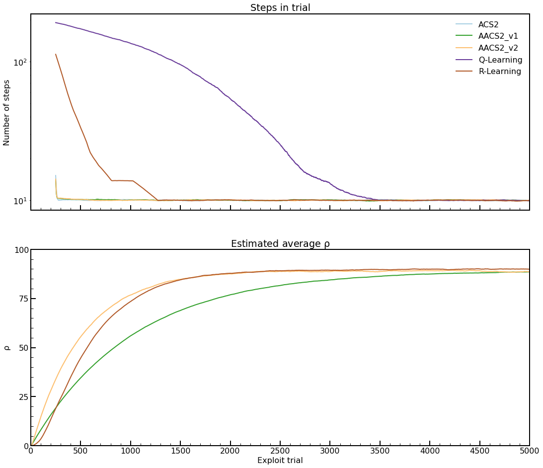
Fig. 5.1 Performance in Corridor-20 environment. Plots averaged over 50 independent runs. Number of steps in exploit trials is averaged over 250 last data points.¶

Payoff Landscape

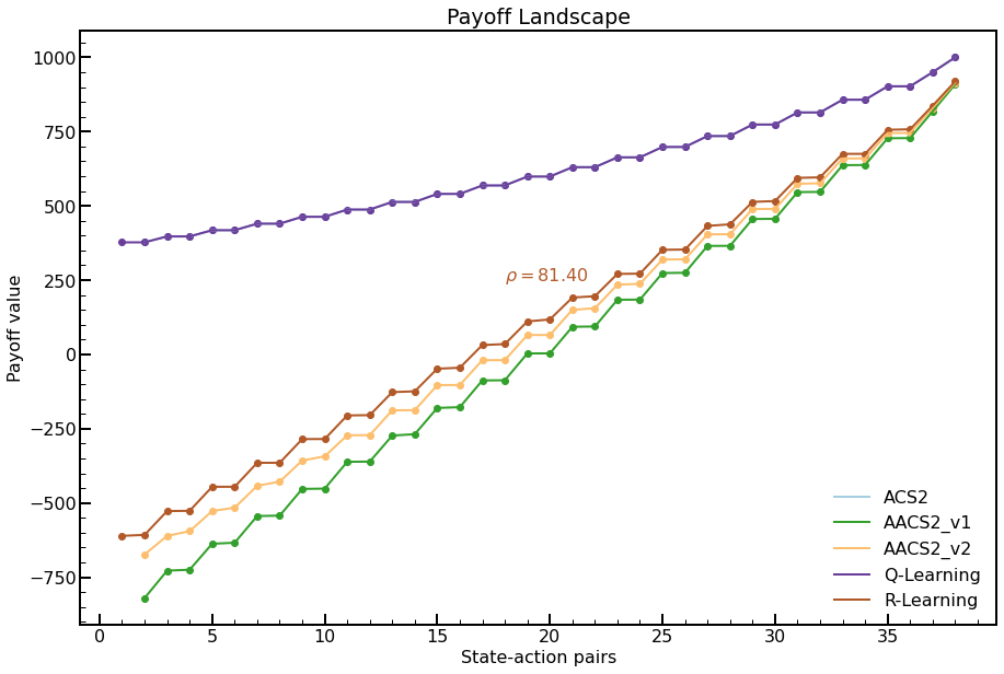
Fig. 5.2 Payoff Landscape for Corridor-20 environment. Payoff values were obtained after 10000 trials. For the Q-Learning and R-Learning, the same learning parameters were applied. The ACS2 and Q-Learning generate exactly the same payoffs for each state-action pair.¶

Statistical verification¶

To statistically assess the population size, the posterior data distribution was modelled using 50 metric values collected in the last trial and then sampled with 100,000 draws.

def build_models(dfs: Dict[str, pd.DataFrame], field: str, query_condition: str):
    results = {}

    for name, df in dfs.items():
        data_arr = df.query(query_condition)[field].to_numpy()
        bayes_model = bayes_estimate(data_arr)
        results[name] = (bayes_model['mu'], bayes_model['std'])

    return results


experiments_data = {
    'corridor20_acs2': corridor20_acs2_metrics.query('agent == "ACS2"'),
    'corridor20_aacs2v1': corridor20_acs2_metrics.query('agent == "AACS2_v1"'),
    'corridor20_aacs2v2': corridor20_acs2_metrics.query('agent == "AACS2_v2"'),
    'corridor20_qlearning': pd.DataFrame(q_learning_runs[0]),
    'corridor20_rlearning': pd.DataFrame(r_learning_runs[0]),
    
    'corridor40_acs2': corridor40_acs2_metrics.query('agent == "ACS2"'),
    'corridor40_aacs2v1': corridor40_acs2_metrics.query('agent == "AACS2_v1"'),
    'corridor40_aacs2v2': corridor40_acs2_metrics.query('agent == "AACS2_v2"'),
    'corridor40_qlearning': pd.DataFrame(q_learning_runs[1]),
    'corridor40_rlearning': pd.DataFrame(r_learning_runs[1]),
    
    'corridor100_acs2': corridor100_acs2_metrics.query('agent == "ACS2"'),
    'corridor100_aacs2v1': corridor100_acs2_metrics.query('agent == "AACS2_v1"'),
    'corridor100_aacs2v2': corridor100_acs2_metrics.query('agent == "AACS2_v2"'),
    'corridor100_qlearning': pd.DataFrame(q_learning_runs[2]),
    'corridor100_rlearning': pd.DataFrame(r_learning_runs[2]),
}

@get_from_cache_or_run(cache_path=f'{cache_dir}/corridor/bayes/steps.dill')
def build_steps_models(dfs: Dict[str, pd.DataFrame]):
    return build_models(dfs, field='steps_in_trial', query_condition=f'trial == {trials - 1}')

@get_from_cache_or_run(cache_path=f'{cache_dir}/corridor/bayes/rho.dill')
def build_rho_models(dfs: Dict[str, pd.DataFrame]):
    filtered_dfs = {}
    for k, v in dfs.items():
        if any(r_model for r_model in ['aacs2v1', 'aacs2v2', 'rlearning'] if k.endswith(r_model)):
            filtered_dfs[k] = v

    return build_models(filtered_dfs, field='rho', query_condition=f'trial == {trials - 1}')

steps_models = build_steps_models(experiments_data)
rho_models = build_rho_models(experiments_data)

def print_bayes_table(name_prefix, steps_models, rho_models):
    print_row = lambda r: f'{round(r[0].mean(), 2)} ± {round(r[0].std(), 2)}'
    rho_data = [print_row(v) for name, v in rho_models.items() if name.startswith(name_prefix)]

    bayes_table_data = [
        ['steps in last trial'] + [print_row(v) for name, v in steps_models.items() if name.startswith(name_prefix)],
        ['average reward per step', '-', rho_data[0], rho_data[1], '-', rho_data[2]]
    ]

    table = tabulate(bayes_table_data,
                     headers=['', 'ACS2', 'AACS2v1', 'AACS2v2', 'Q-Learning', 'R-Learning'],
                     tablefmt="html", stralign='center')
    return HTML(table)

# add glue outputs
glue('51-corridor20-bayes', print_bayes_table('corridor20', steps_models, rho_models), display=False)
glue('51-corridor40-bayes', print_bayes_table('corridor40', steps_models, rho_models), display=False)
glue('51-corridor100-bayes', print_bayes_table('corridor100', steps_models, rho_models), display=False)

Corridor 20

	ACS2	AACS2v1	AACS2v2	Q-Learning	R-Learning
steps in last trial	9.61 ± 0.84	9.54 ± 0.84	9.0 ± 0.82	7.91 ± 0.79	9.31 ± 0.9
average reward per step	-	88.52 ± 0.16	88.65 ± 0.29	-	89.9 ± 0.19

Corridor 40

	ACS2	AACS2v1	AACS2v2	Q-Learning	R-Learning
steps in last trial	19.42 ± 1.65	19.43 ± 1.7	19.47 ± 1.46	124.96 ± 14.21	17.64 ± 1.67
average reward per step	-	44.7 ± 0.14	44.7 ± 0.19	-	44.93 ± 0.12

Corridor 100

	ACS2	AACS2v1	AACS2v2	Q-Learning	R-Learning
steps in last trial	55.95 ± 4.13	51.25 ± 4.19	49.83 ± 4.48	200.0 ± 0.0	48.65 ± 4.37
average reward per step	-	17.84 ± 0.09	17.75 ± 0.13	-	17.85 ± 0.07

Observations¶

The average number of steps can be calculated \(\frac{\sum_0^{n} n}{n-1}\), where \(n\) is the number of distinct Corridor states. For the tested environment it gives the approximate value of \(11.05\), therefore the average reward per step estimation should be close to \(1000 / 11.05 = 90.49\), which corresponds to the Figure 5.1.

The same Figure demonstrates that all investigated agents learned the environments. The anticipatory classifier systems obtained an optimal number of steps after the same number of exploit trials, which is about 200. In addition, the AACS2-v2 updates the \(\rho\) value more aggressively in earlier phases, but the estimate converges near the optimal reward per step.

For the payoff-landscape in Figure 5.2, all allowed state–action pairs were identified in the environment (38 in this case). The final population of learning classifiers was established after 100 trials and was the same size. Both Q-table and R-learning tables were populated using the same parameters and number of trials.

The relative distance between adjacent state-action pairs can be divided into three groups. The first one relates to the discounted reward agents (ACS2, Q-Learning). Both generate almost a similar reward payoff for each state–action. Later, there is the R-Learning algorithm, which estimates the \(\rho\) value and separates states evenly. Furthermore, two AACS2 agents are performing very similarly. The \(\rho\) value calculated by the R-Learning algorithm is lower than the average estimation by the AACS2 algorithm.

Scaled problem instances revealed interesting properties:

the Q-Learning algorithm was not capable of executing the optimal number of steps in environments with \(n=40\), \(n=100\),
for the most challenging problem of \(n=1000\), the AACS2 modification yield better performance than ACS2,
all algorithms with undiscounted reward critera managed to calculate the average reward \(\rho\)

Real-valued Anticipatory Classifier System

Experiment 1 - Straight Corridor

Contents

Experiment 1 - Straight Corridor¶

Results¶

Statistical verification¶

Observations¶