2.5. Overview of the selected environments¶

The range of problem domains to which ALCS can be broadly divided into two categories: classification problems and reinforcement learning problems [122]. Classification problems seek to find a compact set of rules that classify all problem instances with maximal accuracy. They frequently rely on supervised learning, where feedback is provided instantly. The Reinforcement Learning problems seek to find an optimal behavioural policy represented by a compact set of rules. These problems are typically distinguished by inconsistent environmental rewards, requiring multiple actions before a reward is obtained. They can be further discriminated by having Markov properties [53] [123] [124].

This section describes six single- and multi-steps environments used in further experiments. All of them are stationary, Markov toy-problems exhibiting real-valued properties facilitating the evaluation of modifications of anticipatory systems. Most of the environments were used as benchmarks in other works related to measuring the performance of the LCS; however, the Cart Pole environment was never used in this class of algorithms before.

All the mentioned environments pose the standardized interface for enabling the agent to interact with it in a consistent manner [125]. After executing an action, the agent is presented with the current observation (that is not equal to its internal state), possible reward from previously executed action, and whether the interaction is finished. In most cases, a specific reward state acts as an incentive, motivating the forager to reach it.

Corridor¶

The corridor is a 1D multi-step, linear environment introduced by Lanzi to evaluate the XCSF agent [103]. The system output is defined over a finite discrete interval \([0,n]\). On each trial, the agent is placed randomly on the path and can execute two possible actions - move left or right (which corresponds to moving one unit in a particular direction - see Figure 2.11.

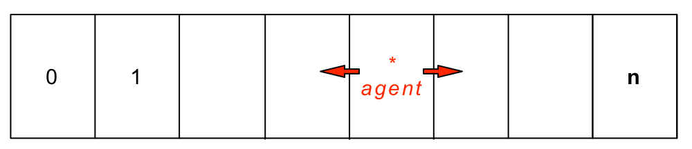
Fig. 2.11 The Corridor environment. The size of the input space is \(n\).¶

Lanzi used a real-valued version of this environment where the agent location is elucidated by a value between \([0,1]\). Predefined step size was added to the current position when it executed an action, thus changing its value. When the agent reaches the final state \(s = 1.0\), the reward is paid out.

The environment examined herein signifies the state already in discretized form, available in three preconfigured sizes with increasing difficulty. The main challenge for the agent here is mainly to learn the reward distribution in possibly long action chains successfully.

Reward scheme: The trial ends when it reaches the final state \(n\) (obtaining reward \(r=1000\)) or when the maximum number of 200 steps in each episode is exceeded. Otherwise, the reward after each step is \(r=0\).

Grid¶

Grid refers to an extension of the Corridor environment [103]. A vertical dimension and two new actions (move up, move down) are added. The raw agent perception is now identified as a pair of real numbers \((s_0, s_1)\), where \(s \in [0,1]\). Similarly, the environment is presented to the agent in a discretized form. Each dimension is divided into \(n-1\) equally spaced buckets - see Figure 2.12.

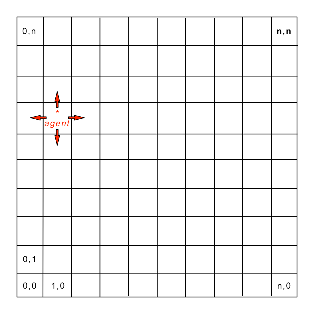
Fig. 2.12 The Grid environment. The size of the input space is \(n^2\). The agent can change its position by moving in four different directions.¶

Reward scheme: The trial ends with reward \(r=1000\) when the final state \((n, n)\) is reached. Otherwise, the reward after each step is \(r=0\). Additionally, the episode is terminated after exceeding the maximum number of 2000 steps.

Real Multiplexer¶

import gym_multiplexer  # noqa: F401

rmpx6bit_env = gym.make('real-multiplexer-6bit-v0')
random_state = rmpx6bit_env.reset()

threshold = 0.5  # secret knowledge

t = HTML(tabulate([
    ['<b>rMPX output</b>'] + [round(s, 2) for s in random_state],
    ['<b>MPX output</b>'] + list(map(lambda x: 1 if x > threshold else 0, random_state))
], tablefmt='unsafehtml', stralign='right'))

glue('rmpx_mpx_mapping_table', t, display=False)

Wilson modified the traditional Boolean Multiplexer (MPX) [32], called Real Multiplexer (rMPX), to examine the performance in single-step environments using real-valued data.

The Boolean n-bit multiplexer defines a set of single-step supervised learning problems conceptually based on an electronic device taking multiple inputs and switching them to the single output. A random, fixed binary string of predefined length is generated in each trial. It comprises two parts - the address and register segments. The first one points to a specific register address that is considered to be a truth value - Figure 2.13 describes the process. This environment is also exciting because it possesses the properties of epistasis and heterogeneity, which are often present within real-world problems such as bioinformatics, finance or behaviour modelling.

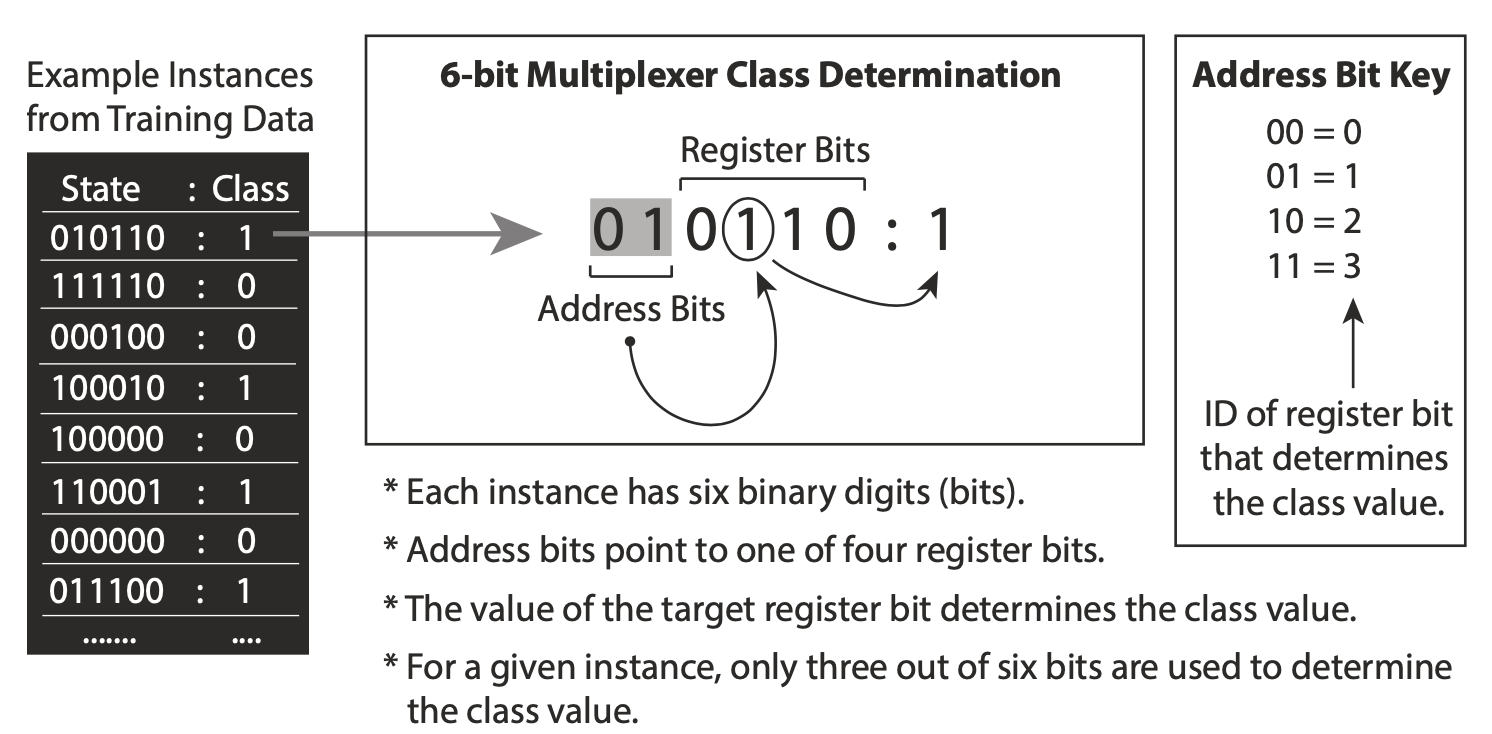
Fig. 2.13 Visualization of determining the output value of 6-bit multiplexer. The address bit points to the first value of the register array that is considered the true output. Diagram taken from [126].¶

For the rMPX, the only difference between a boolean multiplexer is that generated perception consists of real values drawn from a uniform distribution. To validate the correct answer, the additional variable - secret threshold \(\theta = 0.5\) is used to map each allele into binary form. See Table 2.14 for the example of such mapping.

rMPX output	0.48	0.29	0.11	0.86	0.43	0.48	0
MPX output	0	0	0	1	0	0	0

Fig. 2.14 Example of mapping a random 6-bit rMPX output into MPX problem. A threshold of \(\theta=0.5\) was used. The last bit is set to \(0\) as an initial value that will be changed to \(1\) after performing the correct action.¶

However, the standard version is still not suitable to be used with ALCS. Because an agent utilizes perceptual causality to form new classifiers, assuming that after executing an action, the state will change. The MPX does not have any possibility to send feedback about the correctness of the action. Butz suggested two solutions to this problem [26]. In this work, the assumption is that the state generated by the rMPX is extended by one extra bit, denoting whether the classification was successful. This bit is by default set to zero. When the agent responds correctly, it is being switched, thus providing direct feedback. A detailed example can be found in [127].

Reward scheme: If the correct answer is given, the reward \(r=1000\) is paid out, otherwise \(r=0\).

Checkerboard¶

def plot_checkerboard(plot_filename=None):
    import gym_checkerboard  # noqa: F401
    checkerboard_env = gym.make('checkerboard-2D-3div-v0')
    checkerboard_env.reset()

    np_board = checkerboard_env.env._board.board

    fig = plt.figure(figsize=(7, 7))
    ax = fig.add_subplot(111)

    ax.matshow(np_board, cmap=plt.get_cmap('gray_r'), extent=(0, 1, 0, 1), alpha=.5)
    ax.set_xlabel("x")
    ax.set_ylabel("y")

    if plot_filename:
        fig.savefig(plot_filename, dpi=PLOT_DPI)

    return fig

glue('checkerboard-env', plot_checkerboard(f'{plot_dir}/checkerboard-env-visualization.png'), display=False)

The Checkerboard is a single-step environment introduced by Stone in [34]. It was proposed to circumvent certain limitations of the Real Multiplexer when using the interval predicates approach. Because the rMPX problem can be solved by using just a hyperplane decision surface, it is not considered to represent arbitrary intervals in solution space. In order to solve the Checkerboard problem, a hyper-rectangle decision surface is needed for modelling certain interval regions.

This environment works by dividing the \(n\)-dimensional solution space into equal-sized hypercubes. Each hypercube is assigned a white or black color (alternating in all dimensions), see Figure 2.15. The problem difficulty can be controlled by changing the dimensionality \(n\) and the number of divisions in each dimension \(n_d\). In order to allow the colours to be alternating, \(n_d\) must be an odd number.

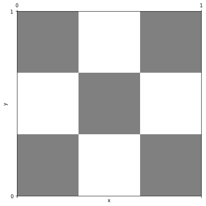
Fig. 2.15 2-dimensional Checkerboard problem with \(n_d=3\). Precise interval predicates are needed for representing selected regions.¶

In each trial, the environment presents a vector of length \(n_d\) or real numbers in the interval \([0, 1)\), representing a point in the solution space. The agent’s goal is to guess the correct colour by performing one of two actions depending on a pointed hypercube’s colour (black or white).

Reward scheme: When the correct answer is given, the reward \(r=1\) is paid out, otherwise \(r=0\).

Cart Pole¶

Barto introduced the Cart Pole environment as a reinforcement learning control problem [128]. The task is to balance a pole that is hinged to a movable cart by applying forces (move left or move right) to the cart’s base (Figure 2.16). The system starts upright, and its goal is to prevent the stick from falling over.

Fig. 2.16 The Cart Pole environment. The goal is to maintain the pole upright for a maximum number of trials.¶

The observation returned by the environment is a vector of four elements - presented in Table 2.1. The challenge for the agent is that each attribute has a specific range of possible values, and two of them additionally span the whole search space.

Table 2.1 Agent’s observation of the Cart Pole environment¶
Attribute	Observation	Min	Max
\(\sigma_0\)	Cart Position	-2.4	2.4
\(\sigma_1\)	Cart Velocity	\(-\infty\)	\(\infty\)
\(\sigma_2\)	Pole Angle	\(\sim\)-41.8°	\(\sim\)41.8°
\(\sigma_3\)	Pole Velocity at Tip	\(-\infty\)	\(\infty\)

The environment is considered solved if the average reward is greater than or equal to 195 over the last 100 trials.

Reward scheme: After each step, a reward of +1 is provided. The episode ends when the pole is more than 15 degrees from vertical or the cart moves more than 2.4 units from the centre.

Finite State World¶

Barry introduced the Finite State World (FSW) [129] environment to investigate the limits of XCS performance in long multi-step environments with a delayed reward. It consists of nodes and directed edges joining the nodes. Each node represents a distinct environmental state and is labelled with a unique state identifier. Each edge represents a possible transition path from one node to another and is also labelled with the action(s) that will cause the movement. An edge can also lead back to the same node. The graph layout used in the experiments is presented in Figure 2.17.

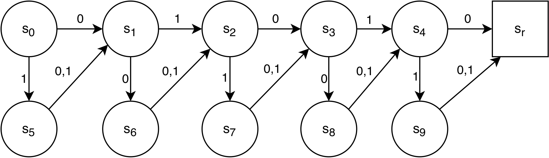
Fig. 2.17 A Finite State World of length 5 (FSW-5). The environment is especially suited for measuring reward propagation for long action chains. Each trial always starts in state \(s_0\), and the agent’s goal is to reach the final state \(s_r\).¶

Although the environment does not expose any real-valued state, it can be treated as a further extension of a discretized Corridor. Most importantly, the challenge is that the agent is presented with the sub-optimal route at every step, which slows for the pursuit of the reward. Additionally, the environment is easily scalable - changing the number of nodes will change the total action chain length.

Reward scheme: A of reward \(r = 100\) is provided when agent reaches final state \(s_r\), otherwise \(r=0\).

Real-valued Anticipatory Classifier System

Overview of the selected environments

Contents