Experiment 3 - Balancing the pole
Contents
import pathlib
from typing import List, Tuple, Dict

import gym
import matplotlib.pyplot as plt
import pandas as pd
from IPython.display import HTML
from lcs.agents.acs2 import Configuration, ACS2
from lcs.metrics import population_metrics
from lcs.strategies.action_selection import EpsilonGreedy, ActionDelay, KnowledgeArray
from myst_nb import glue
from tabulate import tabulate

from src.bayes_estimation import bayes_estimate
from src.commons import NUM_EXPERIMENTS
from src.decorators import repeat, get_from_cache_or_run
from src.metrics import parse_experiments_results
from src.utils import build_plots_dir_path, build_cache_dir_path
from src.visualization import biased_exploration_colors, PLOT_DPI

COLORS = biased_exploration_colors()

plt.ioff()  # turn off interactive plotting

root_dir = pathlib.Path().cwd().parent.parent.parent
cwd_dir = pathlib.Path().cwd()

plot_dir = build_plots_dir_path(root_dir) / cwd_dir.name
cache_dir = build_cache_dir_path(root_dir) / cwd_dir.name


def run_experiment(env_provider, explore_trials, exploit_trials, **conf):
    env = env_provider()
    env.reset()

    cfg = Configuration(**conf)

    explorer = ACS2(cfg)
    metrics_explore = explorer.explore(env, explore_trials)

    exploiter = ACS2(cfg, explorer.population)
    metrics_exploit = explorer.exploit(env, exploit_trials)

    # Parse results into DataFrame
    metrics_df = parse_experiments_results(metrics_explore, metrics_exploit, cfg.metrics_trial_frequency)

    return metrics_df


def average_experiment_runs(runs_dfs: List[pd.DataFrame]) -> pd.DataFrame:
    return pd.concat(runs_dfs).groupby(['trial', 'phase']).mean().reset_index(level='phase')


def plot_cp(epsilon_greedy_df, action_delay_df, knowledge_array_df, op_initial_df, explore_trials, buckets, plot_filename=None):
    fig = plt.figure(figsize=(14, 10))

    # Plots layout
    gs = fig.add_gridspec(2, 1, hspace=.4)
    ax1 = fig.add_subplot(gs[0])
    ax2 = fig.add_subplot(gs[1])

    # Global title
    fig.suptitle(f'Performance of CartPole environment discretized with {buckets} buckets', fontsize=24)

    # Each axis
    ma_window = 5  # moving average window

    # Steps in trial
    epsilon_greedy_df['steps_in_trial'].rolling(window=ma_window).mean().plot(label='Epsilon Greedy', c=COLORS['eg'], ax=ax1)
    action_delay_df['steps_in_trial'].rolling(window=ma_window).mean().plot(label='Action Delay', c=COLORS['ad'], ax=ax1)
    knowledge_array_df['steps_in_trial'].rolling(window=ma_window).mean().plot(label='Knowledge Array', c=COLORS['ka'], ax=ax1)
    op_initial_df['steps_in_trial'].rolling(window=ma_window).mean().plot(label='Optimistic Initial Quality', c=COLORS['oiq'], ax=ax1)

    ax1.axvline(x=explore_trials, color='red', linewidth=1, linestyle="--")
    ax1.axhline(y=195, color='black', linewidth=1, linestyle="--")

    ax1.set_xlabel('Trial')
    ax1.set_ylabel('Steps')
    ax1.set_title(f'Steps in each trial')
    ax1.set_ylim(0, 200)

    # Population
    epsilon_greedy_df['reliable'].rolling(window=ma_window).mean().plot(label='Epsilon Greedy', c=COLORS['eg'], ax=ax2)
    action_delay_df['reliable'].rolling(window=ma_window).mean().plot(label='Action Delay', c=COLORS['ad'], ax=ax2)
    knowledge_array_df['reliable'].rolling(window=ma_window).mean().plot(label='Knowledge Array', c=COLORS['ka'], ax=ax2)
    op_initial_df['reliable'].rolling(window=ma_window).mean().plot(label='Optimistic Initial Quality', c=COLORS['oiq'], ax=ax2)

    ax2.axvline(x=explore_trials, color='red', linewidth=1, linestyle="--")

    ax2.set_xlabel('Trial')
    ax2.set_ylabel('Classifiers')
    ax2.set_title(f'Reliable classifiers')

    # Create legend
    handles, labels = ax2.get_legend_handles_labels()
    fig.legend(handles, labels, loc='lower center', ncol=4)

    if plot_filename:
        fig.savefig(plot_filename, dpi=PLOT_DPI)

    return fig


# settings
USE_RAY = True
explore_trials, exploit_trials = 500, 500

# Bucket configurations
buckets_v1 = (1, 1, 6, 6)
buckets_v2 = (4, 4, 4, 4)
buckets_v3 = (2, 2, 6, 6)
buckets_v4 = (1, 2, 4, 4)
buckets_v5 = (1, 1, 8, 8)

glue('41_e3_explore_trials', explore_trials, display=False)
glue('41_e3_exploit_trials', exploit_trials, display=False)
Experiment 3 - Balancing the pole
The challenging part about the Cart Pole problem is that attributes from the perception vector are described with different scales. Moreover, two of them range to infinity. This situation might occur when applying the ALCS agent to the real-world domain.
Splitting each attribute into a fixed amount of buckets is infeasible. Proposed solution involved assigning maximum, experienced values for both the cart \(\sigma_1\) and pole \(\sigma_3\) velocity. In this case:
cart velocity \(\sigma_1 \in [-0.5, 0.5]\),
pole velocity at tip \(\sigma_3 \in [-3500, 3500]\)
Additionally, a specific discretizer was used to divide each attribute into a predefined number of bins. This procedure implies precautions when performing the cross-over operation; therefore, it was disabled.
The experiment analyzes both the impact of selecting the granularity of the discretization scheme and the biased exploration technique. The ACS2 agent is first executing 500 explore trials using a specific method and then tries to use gained knowledge by selecting best action in further 500 exploit trials.
Five different discretization schemes chosen arbitrarily, defining a number of bins per attribute are listed below:
1, 1, 6, 6,4, 4, 4, 4,2, 2, 6, 6,1, 2, 4, 4,1, 1, 8, 8
The metrics of reliable population size and actual performance were both depicted in Figure 4.6 and estimated probabilistically for the above-mentioned schemes.
class CartPoleObservationWrapper(gym.ObservationWrapper):
    # https://medium.com/@tuzzer/cart-pole-balancing-with-q-learning-b54c6068d947
    # _high = [env.observation_space.high[0], 0.5, env.observation_space.high[2], math.radians(50)]
    # _low = [env.observation_space.low[0], -0.5, env.observation_space.low[2], -math.radians(50)]
    def __init__(self, env, buckets):
        super().__init__(env)
        self._high = [env.observation_space.high[0], 0.5, env.observation_space.high[2], 3500]
        self._low = [env.observation_space.low[0], -0.5, env.observation_space.low[2], -3500]
        self._buckets = buckets

    def observation(self, obs):
        ratios = [(obs[i] + abs(self._low[i])) / (self._high[i] - self._low[i]) for i in range(len(obs))]
        new_obs = [int(round((self._buckets[i] - 1) * ratios[i])) for i in range(len(obs))]
        new_obs = [min(self._buckets[i] - 1, max(0, new_obs[i])) for i in range(len(obs))]
        return [str(o) for o in new_obs]


def cp_env_provider(buckets: Tuple[int]):
    return CartPoleObservationWrapper(gym.make('CartPole-v0'), buckets)


def cp_metrics(agent, env):
    pop = agent.population
    metrics = {}
    metrics.update(population_metrics(pop, env))
    return metrics


cp_base_params = {
    "classifier_length": 4,
    "number_of_possible_actions": 2,
    "epsilon": 0.9,
    "beta": 0.01,
    "gamma": 0.995,
    "initial_q": 0.5,
    "theta_exp": 50,
    "theta_ga": 50,
    "do_ga": True,
    "chi": 0.0,
    "mu": 0.03,
    "metrics_trial_frequency": 1,
    "user_metrics_collector_fcn": cp_metrics
}


def buckets_to_str(buckets, delimiter='_'):
    return f'{delimiter.join(map(str, buckets))}'


def run_cart_pole_biased_exploration(buckets):
    env_provider = lambda: cp_env_provider(buckets)

    eg = run_experiment(env_provider, explore_trials, exploit_trials, **(cp_base_params | {'action_selector': EpsilonGreedy}))
    ad = run_experiment(env_provider, explore_trials, exploit_trials, **(cp_base_params | {'action_selector': ActionDelay, 'biased_exploration_prob': 0.5}))
    ka = run_experiment(env_provider, explore_trials, exploit_trials, **(cp_base_params | {'action_selector': KnowledgeArray, 'biased_exploration_prob': 0.5}))
    oiq = run_experiment(env_provider, explore_trials, exploit_trials, **(cp_base_params | {'action_selector': EpsilonGreedy, 'biased_exploration_prob': 0.8}))

    return eg, ad, ka, oiq


@get_from_cache_or_run(cache_path=f'{cache_dir}/cart_pole/{buckets_to_str(buckets_v1)}.dill')
@repeat(num_times=NUM_EXPERIMENTS, use_ray=USE_RAY)
def cp_buckets_v1():
    return run_cart_pole_biased_exploration(buckets_v1)


@get_from_cache_or_run(cache_path=f'{cache_dir}/cart_pole/{buckets_to_str(buckets_v2)}.dill')
@repeat(num_times=NUM_EXPERIMENTS, use_ray=USE_RAY)
def cp_buckets_v2():
    return run_cart_pole_biased_exploration(buckets_v2)


@get_from_cache_or_run(cache_path=f'{cache_dir}/cart_pole/{buckets_to_str(buckets_v3)}.dill')
@repeat(num_times=NUM_EXPERIMENTS, use_ray=USE_RAY)
def cp_buckets_v3():
    return run_cart_pole_biased_exploration(buckets_v3)


@get_from_cache_or_run(cache_path=f'{cache_dir}/cart_pole/{buckets_to_str(buckets_v4)}.dill')
@repeat(num_times=NUM_EXPERIMENTS, use_ray=USE_RAY)
def cp_buckets_v4():
    return run_cart_pole_biased_exploration(buckets_v4)


@get_from_cache_or_run(cache_path=f'{cache_dir}/cart_pole/{buckets_to_str(buckets_v5)}.dill')
@repeat(num_times=NUM_EXPERIMENTS, use_ray=USE_RAY)
def cp_buckets_v5():
    return run_cart_pole_biased_exploration(buckets_v5)


def extract(experiment_runs):
    eg_dfs, ad_dfs, ka_dfs, oiq_dfs = [], [], [], []

    for eg_df, ad_df, ka_df, oiq_df in experiment_runs:
        eg_dfs.append(eg_df)
        ad_dfs.append(ad_df)
        ka_dfs.append(ka_df)
        oiq_dfs.append(oiq_df)

    return eg_dfs, ad_dfs, ka_dfs, oiq_dfs


# Run the calculations
cp_bv1_eg_dfs, cp_bv1_ad_dfs, cp_bv1_ka_dfs, cp_bv1_oiq_dfs = extract(cp_buckets_v1())
cp_bv2_eg_dfs, cp_bv2_ad_dfs, cp_bv2_ka_dfs, cp_bv2_oiq_dfs = extract(cp_buckets_v2())
cp_bv3_eg_dfs, cp_bv3_ad_dfs, cp_bv3_ka_dfs, cp_bv3_oiq_dfs = extract(cp_buckets_v3())
cp_bv4_eg_dfs, cp_bv4_ad_dfs, cp_bv4_ka_dfs, cp_bv4_oiq_dfs = extract(cp_buckets_v4())
cp_bv5_eg_dfs, cp_bv5_ad_dfs, cp_bv5_ka_dfs, cp_bv5_oiq_dfs = extract(cp_buckets_v5())

# Plot visualization
glue('41-e3-cartpole-fig',
     plot_cp(
         average_experiment_runs(cp_bv1_eg_dfs),
         average_experiment_runs(cp_bv1_ad_dfs),
         average_experiment_runs(cp_bv1_ka_dfs),
         average_experiment_runs(cp_bv1_oiq_dfs),
         explore_trials=explore_trials,
         buckets=buckets_v1,
         plot_filename=f'{plot_dir}/cartpole-performance.png'),
     display=False)
Results
ACS2 parameters
\(\beta=0.01\), \(\gamma = 0.995\), \(\theta_r = 0.9\), \(\theta_i=0.1\), \(\epsilon = 0.9\) \(\theta_{GA} = 50\), \(\theta_{AS}=20\), \(\theta_{exp}=50\), \(m_u=0.03\), \(u_{max}=4\), \(\chi=0.0\).
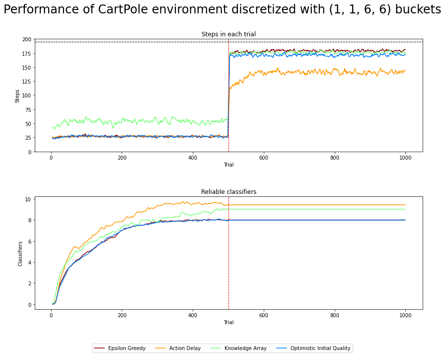
Fig. 4.6 Performance in CartPole environment. 500 exploration and 500 exploitation trials averaged over 50 runs. Moving average of 5 last trials applied for clarity. The dotted vertical line indicates the execution of explore and exploit phases. The environment is considered solved if the average reward is greater than or equal to 195 over the last 100 trials.
Statistical verification
To statistically assess the population size, the posterior data distribution was modelled using 50 metric values collected in the last trial and then sampled with 100,000 draws. For the obtained reward, the average value from exploit trials is considered a representative state of algorithm performance.
experiments_data = {
    buckets_v1: [cp_bv1_eg_dfs, cp_bv1_ad_dfs, cp_bv1_ka_dfs, cp_bv1_oiq_dfs],
    buckets_v2: [cp_bv2_eg_dfs, cp_bv2_ad_dfs, cp_bv2_ka_dfs, cp_bv2_oiq_dfs],
    buckets_v3: [cp_bv3_eg_dfs, cp_bv3_ad_dfs, cp_bv3_ka_dfs, cp_bv3_oiq_dfs],
    buckets_v4: [cp_bv4_eg_dfs, cp_bv4_ad_dfs, cp_bv4_ka_dfs, cp_bv4_oiq_dfs],
    buckets_v5: [cp_bv5_eg_dfs, cp_bv5_ad_dfs, cp_bv5_ka_dfs, cp_bv5_oiq_dfs]
}


def train_bayes_model(dfs, query_condition, field):
    data_arr = pd.concat(dfs).query(query_condition)[field].to_numpy()
    bayes_model = bayes_estimate(data_arr)
    return bayes_model['mu'], bayes_model['std']


def build_models(dfs: Dict, field: str, query_condition: str):
    results = {}

    for bucket, dfs in dfs.items():
        posteriors = [train_bayes_model(df, query_condition, field) for df in dfs]
        results[bucket] = posteriors

    return results


def print_bayes_table(data):
    table_data = [[buckets_to_str(bucket, ',')] + rewards for bucket, rewards in data.items()]

    table = tabulate(table_data,
                     headers=['', 'Epsilon Greedy', 'Action Delay', 'Knowledge Array', 'Optimistic Initial Quality'],
                     tablefmt="html", stralign='right', floatfmt=".2f")

    return HTML(table)


print_row = lambda r: f'{round(r[0].mean(), 2)} ± {round(r[0].std(), 2)}'

# Average Steps in exploit phase
avg_reward = lambda dfs: pd.concat(dfs).query('phase == "exploit"')['steps_in_trial'].mean()

average_rewards_data = {}
for bucket, dfs in experiments_data.items():
    average_rewards_data[bucket] = list(map(avg_reward, dfs))


# reliable classifiers
@get_from_cache_or_run(cache_path=f'{cache_dir}/cart_pole/bayes/reliable.dill')
def build_reliable_models(dfs: Dict):
    return build_models(dfs, field='reliable', query_condition=f'trial == {explore_trials - 1}')


# run computations
reliable_data = build_reliable_models(experiments_data)

reliable_table_data = {}
for bucket, models in reliable_data.items():
    reliable_table_data[bucket] = list(map(print_row, models))

# Add glue objects
glue('average_steps', print_bayes_table(average_rewards_data), display=False)
glue('bayes_reliable_classifies', print_bayes_table(reliable_table_data), display=False)
Epsilon Greedy Action Delay Knowledge Array Optimistic Initial Quality 1,1,6,6 178.40 138.69 175.72 171.20 4,4,4,4 18.85 19.14 20.34 18.56 2,2,6,6 59.73 44.58 95.68 60.72 1,2,4,4 133.93 150.62 128.70 132.36 1,1,8,8 181.61 154.09 172.75 176.42
Epsilon Greedy Action Delay Knowledge Array Optimistic Initial Quality 1,1,6,6 8.0 ± 0.0 9.39 ± 0.18 9.01 ± 0.23 8.0 ± 0.0 4,4,4,4 6.33 ± 0.26 4.38 ± 0.19 5.65 ± 0.23 6.06 ± 0.23 2,2,6,6 6.99 ± 0.25 7.29 ± 0.25 8.27 ± 0.33 7.48 ± 0.31 1,2,4,4 11.23 ± 0.18 9.83 ± 0.18 10.01 ± 0.18 10.86 ± 0.22 1,1,8,8 9.14 ± 0.12 8.92 ± 0.12 10.42 ± 0.21 9.18 ± 0.14
Observations
Surprisingly, when using the discretization of 1, 1, 6, 6, the agent can keep the pole upright for about 175 steps in each trial after performing just 500 learning trials. This score was possible for every method except the AD. On the other side, AD created more reliable classifiers quicker than other methods.
The experiment’s performance turned out to be very sensitive to the discretization bins chosen. For example, a slightly larger amount of bins for pole angle and velocity (eight bins in both cases) increased the number of upright steps. In official terms, the environment is still not solved. However, it turned out that the number of reliable classifiers required to obtain such a score is less than 10. That allows a very compact and human-readable form of storing knowledge (see Table below for example).
@get_from_cache_or_run(cache_path=f'{cache_dir}/cart_pole/epsilon_greedy_single_run.dill')
def cp_single_run():
    cfg = Configuration(**(cp_base_params | {'action_selector': EpsilonGreedy}))
    agent = ACS2(cfg)
    agent.explore(cp_env_provider(buckets_v1), explore_trials)
    return agent  # only interested in resulting population


# execute run
cp_agent = cp_single_run()

reliable = [cl for cl in cp_agent.population if cl.is_reliable()]
for cl in sorted(reliable, key=lambda cl: -cl.fitness):
    print(
        f'[{cl.condition} {cl.action} {cl.effect}]\t\tmark: {cl.mark}\tquality: {cl.q:.2f}\treward: {cl.r:.2f}\tnumerosity: {cl.num}')
[##23 0 ####]		mark: 00##	quality: 0.96	reward: 3.34	numerosity: 1
[##32 1 ####]		mark: 00##	quality: 0.96	reward: 3.24	numerosity: 1
[##22 1 ####]		mark: 00##	quality: 0.98	reward: 2.78	numerosity: 1
[##33 0 ####]		mark: 00##	quality: 0.95	reward: 2.23	numerosity: 3
[##12 0 ####]		mark: 00##	quality: 0.98	reward: 1.44	numerosity: 1
[##12 1 ####]		mark: empty	quality: 1.00	reward: 1.36	numerosity: 20
[##43 1 ####]		mark: 00##	quality: 0.97	reward: 1.32	numerosity: 6
[##43 0 ####]		mark: empty	quality: 1.00	reward: 1.22	numerosity: 20
It can be seen that the majority of reliable classifiers are marked on the first two attributes, meaning that they too sweep and therefore should be more distinguishable (for example, by increasing discretization). In order to set them properly, a dedicated hyper-parameter optimization process is advised.
Despite fragility, the obtained result is auspicious, showing that ALCS methods can be compared to other highly sophisticated black-box approaches and maintain a highly verbose problem model.
Software packages used
import session_info

session_info.show()
Click to view session information
-----
gym                 0.21.0
lcs                 NA
matplotlib          3.5.1
myst_nb             0.13.1
pandas              1.4.0
session_info        1.0.0
src                 (embedded book's utils module)
tabulate            0.8.9
-----
Click to view modules imported as dependencies
PIL                         8.4.0
arviz                       0.11.2
asttokens                   NA
attr                        21.4.0
babel                       2.9.1
backcall                    0.2.0
beta_ufunc                  NA
binom_ufunc                 NA
brotli                      NA
cachetools                  5.0.0
certifi                     2021.10.08
cffi                        1.15.0
cftime                      1.5.2
charset_normalizer          2.0.10
click                       7.1.2
cloudpickle                 2.0.0
colorama                    0.4.4
colorful                    0.5.4
colorful_orig               0.5.4
cryptography                36.0.1
cycler                      0.10.0
cython_runtime              NA
databricks_cli              NA
dateutil                    2.8.2
debugpy                     1.5.1
decorator                   5.1.1
defusedxml                  0.7.1
dill                        0.3.4
docutils                    0.16
entrypoints                 0.3
executing                   0.8.2
fastprogress                0.2.7
filelock                    3.4.2
google                      NA
greenlet                    1.1.2
grpc                        1.43.0
hiredis                     2.0.0
idna                        3.3
imagesize                   NA
importlib_metadata          NA
ipykernel                   6.7.0
ipython_genutils            0.2.0
ipywidgets                  7.6.5
jedi                        0.18.1
jinja2                      3.0.3
jsonschema                  3.2.0
jupyter_cache               0.4.3
jupyter_sphinx              0.3.2
jupyterlab_pygments         0.1.2
kiwisolver                  1.3.2
linkify_it                  1.0.3
markdown_it                 1.1.0
markupsafe                  2.0.1
matplotlib_inline           NA
mdit_py_plugins             0.2.8
mistune                     0.8.4
mlflow                      1.23.1
mpl_toolkits                NA
msgpack                     1.0.3
myst_parser                 0.15.2
nbclient                    0.5.10
nbconvert                   6.4.1
nbformat                    5.1.3
nbinom_ufunc                NA
netCDF4                     1.5.8
numpy                       1.22.1
packaging                   21.3
pandocfilters               NA
parso                       0.8.3
pexpect                     4.8.0
pickleshare                 0.7.5
pkg_resources               NA
prompt_toolkit              3.0.26
psutil                      5.9.0
ptyprocess                  0.7.0
pure_eval                   0.2.2
pvectorc                    NA
pydev_ipython               NA
pydevconsole                NA
pydevd                      2.6.0
pydevd_concurrency_analyser NA
pydevd_file_utils           NA
pydevd_plugins              NA
pydevd_tracing              NA
pygments                    2.11.2
pylab                       NA
pymc3                       3.11.4
pyparsing                   3.0.7
pyrsistent                  NA
pytz                        2021.3
ray                         1.9.2
redis                       4.1.2
requests                    2.27.1
scipy                       1.7.3
semver                      2.13.0
setproctitle                1.2.2
setuptools                  60.5.0
six                         1.16.0
socks                       1.7.1
sphinx                      4.4.0
sphinxcontrib               NA
sqlalchemy                  1.4.31
stack_data                  0.1.4
testpath                    0.5.0
theano                      1.1.2
tornado                     6.1
tqdm                        4.62.3
traitlets                   5.1.1
typing_extensions           NA
uc_micro                    1.0.1
unicodedata2                NA
urllib3                     1.26.8
wcwidth                     0.2.5
xarray                      0.21.0
yaml                        6.0
zipp                        NA
zmq                         22.3.0
-----
IPython             8.0.1
jupyter_client      7.1.2
jupyter_core        4.9.1
notebook            6.4.8
-----
Python 3.9.10 | packaged by conda-forge | (main, Feb  1 2022, 21:24:11) [GCC 9.4.0]
Linux-5.13.0-30-generic-x86_64-with-glibc2.31
-----
Session information updated at 2022-02-24 17:06