Experiment 3 - Single-step environment performance
Contents
import itertools
import pathlib
import warnings

import bitstring
import gym
import gym_multiplexer  # noqa: F401
from lcs import Perception
from myst_nb import glue
from tabulate import tabulate
from IPython.display import HTML

from src.bayes_estimation import bayes_estimate
from src.bayes_plotting import plot_bayes_comparison
from src.commons import NUM_EXPERIMENTS
from src.decorators import repeat, get_from_cache_or_run
from src.discretized_experiments import *
from src.utils import build_plots_dir_path, build_cache_dir_path

plt.ioff()  # turn off interactive plotting
plt.style.use('../../../../src/phd.mplstyle')

root_dir = pathlib.Path().cwd().parent.parent.parent.parent
cwd_dir = pathlib.Path().cwd()

plot_dir = build_plots_dir_path(root_dir) / cwd_dir.parent.name / cwd_dir.name
cache_dir = build_cache_dir_path(root_dir) / cwd_dir.parent.name / cwd_dir.name

TRIALS = 15_000
USE_RAY = True

RMPX_BINS = 10
RMPX_SIZE = 3
RMPX_THRESHOLD = 0.5
CTRL_BITS = 1

glue('33_e3_trials', TRIALS, display=False)
glue('33_e3_rmpx_threshold', RMPX_THRESHOLD, display=False)
glue('33_e3_rmpx_bins', RMPX_BINS, display=False)
Experiment 3 - Single-step environment performance
The potential of evolving the internal model of the environment is explored by three ALCS implementations - ACS, ACS2 and YACS. Moreover, two additional enhancements are also explicitly investigated - ACS2 with enabled GA component and traditional Dyna-Q implementation. All the algorithms use similar rule structure and their behaviour can be compared using a set of common metrics of Classifier population size, Knowledge, Generalization and Trial time.
The chosen environment is a single-step, 3-bit Real Multiplexer. The investigation was not carried out for greater perception vectors due to the increased computational complexity required for handling a greater amount of interacting classifiers and calculating the metrics, however with sufficient resources, similar results can also be obtained for larger problem instances.
The agent perceives an observation vector of four real-valued attributes. Then, a \(k\) bins discretizer is used to convert them into integers, where the \(k\) value controls the accuracy of generated rules. Thus, the input space of the environment can be calculated as \(2k^n\), where \(k\) refers to the number of bins and \(n\) is the length of the multiplexer output.
Because the rMPX threshold was set to the value of 0.5, a setting of \(k=2\) bins should be sufficient to model the hyper-plane decision surface. The tests were, however, performed by discretizing each attribute into 10 fixed-sized buckets. The following setting provides excessive-resolution and substantiates the capabilities of real-valued input handling.
In each trial of the experiment, the agent executes the exploration phase for the total of 15000 trials solely. Moreover, to present coherent results and draw statistical inferences, each experiment is repeated 50 times.
rmpx = gym.make(f'real-multiplexer-{RMPX_SIZE}bit-v0')

_range, _low = (rmpx.observation_space.high - rmpx.observation_space.low, rmpx.observation_space.low)

RMPX_STEP = _range / RMPX_BINS


class RealMultiplexerUtils:
    def __init__(self, size, ctrl_bits, bins, _range, _threshold=RMPX_THRESHOLD):
        self._size = size
        self._ctrl_bits = ctrl_bits
        self._bins = bins
        self._step = _range / bins
        self._threshold = _threshold

        self._attribute_values = [list(range(0, bins))] * (size) + [[0, bins]]
        self._input_space = itertools.product(*self._attribute_values)
        self.state_mapping = {idx: s for idx, s in enumerate(self._input_space)}
        self.state_mapping_inv = {v: k for k, v in self.state_mapping.items()}

    def discretize(self, obs, _type=int):
        r = (obs + np.abs(_low)) / _range
        b = (r * RMPX_BINS).astype(int)
        return b.astype(_type).tolist()

    def reverse_discretize(self, discretized):
        return discretized * self._step[:len(discretized)]

    def get_transitions(self):
        transitions = []

        initial_dstates = [list(range(0, self._bins))] * (self._size)
        for d_state in itertools.product(*initial_dstates):
            correct_answer = self._get_correct_answer(d_state)

            if correct_answer == 0:
                transitions.append((d_state + (0,), 0, d_state + (self._bins,)))
                transitions.append((d_state + (0,), 1, d_state + (0,)))
            else:
                transitions.append((d_state + (0,), 0, d_state + (0,)))
                transitions.append((d_state + (0,), 1, d_state + (self._bins,)))

        return transitions

    def _get_correct_answer(self, discretized):
        estimated_obs = self.reverse_discretize(discretized)
        bits = bitstring.BitArray(estimated_obs > self._threshold)
        _ctrl_bits = bits[:self._ctrl_bits]
        _data_bits = bits[self._ctrl_bits:]

        return int(_data_bits[_ctrl_bits.uint])


rmpx_utils = RealMultiplexerUtils(RMPX_SIZE, CTRL_BITS, RMPX_BINS, _range)
# metrics
def generalization_score(pop):
    # Compute proportion of wildcards in classifier condition across all classifiers
    wildcards = sum(1 for cl in pop for cond in cl.condition if cond == '#' or (hasattr(cond, 'symbol') and cond.symbol == '#'))
    all_symbols = sum(len(cl.condition) for cl in pop)
    return wildcards / all_symbols


def rmpx_knowledge(population, env):
    reliable = [c for c in population if c.is_reliable()]
    nr_correct = 0

    for start, action, end in rmpx_utils.get_transitions():
        p0 = Perception([str(el) for el in start])
        p1 = Perception([str(el) for el in end])

        if any([True for cl in reliable if cl.predicts_successfully(p0, action, p1)]):
            nr_correct += 1

    return nr_correct / len(rmpx_utils.get_transitions())


def rmpx_metrics_collector(agent, env):
    population = agent.population
    return {
        'pop': len(population),
        'knowledge': rmpx_knowledge(population, env),
        'generalization': generalization_score(population)
    }


# DynaQ helpers
def rmpx_perception_to_int(p0, discretize=True):
    if discretize:
        p0 = rmpx_utils.discretize(p0)

    return rmpx_utils.state_mapping_inv[tuple(p0)]


def dynaq_rmpx_knowledge_calculator(model, env):
    all_transitions = 0
    nr_correct = 0

    for p0, a, p1 in rmpx_utils.get_transitions():
        s0 = rmpx_perception_to_int(p0, discretize=False)
        s1 = rmpx_perception_to_int(p1, discretize=False)

        all_transitions += 1
        if s0 in model and a in model[s0] and model[s0][a][0] == s1:
            nr_correct += 1

    return nr_correct / len(rmpx_utils.get_transitions())
class DiscretizedWrapper(gym.ObservationWrapper):
    def observation(self, obs):
        return rmpx_utils.discretize(obs, _type=str)


class SingleStateWrapper(DiscretizedWrapper):
    def observation(self, obs):
        return rmpx_utils.state_mapping_inv[tuple(map(int, obs))]


common_params = {
    'classifier_length': RMPX_SIZE + 1,
    'possible_actions': 2,
    'learning_rate': 0.1,
    'metrics_trial_freq': 100,
    'metrics_fcn': rmpx_metrics_collector,
    'trials': TRIALS
}

yacs_params = {
    'trace_length': 3,
    'estimate_expected_improvements': False,
    'feature_possible_values': [{str(i) for i in range(RMPX_BINS)}] * RMPX_SIZE + [{'0', '10'}]
}

dynaq_params = {
    'q_init': np.zeros((len(rmpx_utils.state_mapping), 2)),
    'model_init': {},
    'knowledge_fcn': dynaq_rmpx_knowledge_calculator,
    'epsilon': 0.5
}


@get_from_cache_or_run(cache_path=f'{cache_dir}/rmpx_{RMPX_SIZE}bit/acs.dill')
@repeat(num_times=NUM_EXPERIMENTS, use_ray=USE_RAY)
def run_rmpx_with_acs():
    return single_acs_experiment(
        env_provider=lambda: DiscretizedWrapper(rmpx),
        trials=common_params['trials'],
        classifier_length=common_params['classifier_length'],
        possible_actions=common_params['possible_actions'],
        learning_rate=common_params['learning_rate'],
        metrics_trial_freq=common_params['metrics_trial_freq'],
        metrics_fcn=common_params['metrics_fcn'])


@get_from_cache_or_run(cache_path=f'{cache_dir}/rmpx_{RMPX_SIZE}bit/acs2.dill')
@repeat(num_times=NUM_EXPERIMENTS, use_ray=USE_RAY)
def run_rmpx_with_acs2():
    return single_acs2_experiment(
        env_provider=lambda: DiscretizedWrapper(rmpx),
        trials=common_params['trials'],
        classifier_length=common_params['classifier_length'],
        possible_actions=common_params['possible_actions'],
        learning_rate=common_params['learning_rate'],
        do_ga=False,
        initial_q=0.5,
        metrics_trial_freq=common_params['metrics_trial_freq'],
        metrics_fcn=common_params['metrics_fcn']
    )


@get_from_cache_or_run(cache_path=f'{cache_dir}/rmpx_{RMPX_SIZE}bit/acs2_ga.dill')
@repeat(num_times=NUM_EXPERIMENTS, use_ray=USE_RAY)
def run_rmpx_with_acs2_ga():
    return single_acs2_experiment(
        env_provider=lambda: DiscretizedWrapper(rmpx),
        trials=common_params['trials'],
        classifier_length=common_params['classifier_length'],
        possible_actions=common_params['possible_actions'],
        learning_rate=common_params['learning_rate'],
        do_ga=True,
        initial_q=0.5,
        metrics_trial_freq=common_params['metrics_trial_freq'],
        metrics_fcn=common_params['metrics_fcn']
    )


@get_from_cache_or_run(cache_path=f'{cache_dir}/rmpx_{RMPX_SIZE}bit/yacs.dill')
@repeat(num_times=NUM_EXPERIMENTS, use_ray=USE_RAY)
def run_rmpx_with_yacs():
    return single_yacs_experiment(
        env_provider=lambda: DiscretizedWrapper(rmpx),
        trials=common_params['trials'],
        classifier_length=common_params['classifier_length'],
        possible_actions=common_params['possible_actions'],
        learning_rate=common_params['learning_rate'],
        trace_length=yacs_params['trace_length'],
        estimate_expected_improvements=yacs_params['estimate_expected_improvements'],
        feature_possible_values=yacs_params['feature_possible_values'],
        metrics_trial_freq=common_params['metrics_trial_freq'],
        metrics_fcn=common_params['metrics_fcn']
    )


@get_from_cache_or_run(cache_path=f'{cache_dir}/rmpx_{RMPX_SIZE}bit/dynaq.dill')
@repeat(num_times=NUM_EXPERIMENTS, use_ray=USE_RAY)
def run_rmpx_with_dynaq():
    return single_dynaq_experiment(
        env_provider=lambda: SingleStateWrapper(DiscretizedWrapper(rmpx)),
        trials=common_params['trials'],
        q_init=dynaq_params['q_init'],
        model_init=dynaq_params['model_init'],
        epsilon=dynaq_params['epsilon'],
        learning_rate=common_params['learning_rate'],
        knowledge_fcn=dynaq_params['knowledge_fcn'],
        metrics_trial_freq=common_params['metrics_trial_freq']
    )


@get_from_cache_or_run(cache_path=f'{cache_dir}/corridor/dynaq.dill')
@repeat(num_times=NUM_EXPERIMENTS, use_ray=USE_RAY)
def run_corridor_with_dynaq():
    return single_dynaq_experiment(
        env_provider=lambda: SingleStateWrapper(CorridorObservationWrapper(corridor)),
        trials=common_params['trials'],
        q_init=dynaq_params['q_init'],
        model_init=dynaq_params['model_init'],
        epsilon=dynaq_params['epsilon'],
        learning_rate=common_params['learning_rate'],
        knowledge_fcn=dynaq_params['knowledge_fcn'],
        metrics_trial_freq=common_params['metrics_trial_freq']
    )


# Run computations
rmpx_acs_runs = run_rmpx_with_acs()
rmpx_acs2_runs = run_rmpx_with_acs2()
rmpx_acs2_ga_runs = run_rmpx_with_acs2_ga()
rmpx_yacs_runs = run_rmpx_with_yacs()
rmpx_dynaq_runs = run_rmpx_with_dynaq()

# Collect metrics to single dataframe
metrics_df = pd.concat([
    *[parse_lcs_metrics('acs', metrics) for _, metrics in rmpx_acs_runs],
    *[parse_lcs_metrics('acs2', metrics) for _, metrics in rmpx_acs2_runs],
    *[parse_lcs_metrics('acs2_ga', metrics) for _, metrics in rmpx_acs2_ga_runs],
    *[parse_lcs_metrics('yacs', metrics) for _, metrics in rmpx_yacs_runs],
    *[parse_dyna_metrics('dynaq', metrics) for _, _, metrics in rmpx_dynaq_runs],
])
metrics_df.set_index(['agent', 'trial'], inplace=True)

# Average them by agent and trial
metrics_averaged_df = metrics_df.groupby(['agent', 'trial']).mean()

# plot figure
with warnings.catch_warnings():
    warnings.simplefilter("ignore")
    rmpx3bit_fig = plot_comparison(metrics_averaged_df, plot_filename=f'{plot_dir}/rmpx_3bit_performance.png')
    glue('32_e1_rmpx3bit_discretized_performance_fig', rmpx3bit_fig, display=False)
Results
Common parameters that were used across the experiments included the following: learning rate \(\beta=0.1\), exploration probability \(\epsilon=0.5\), discount factor \(\gamma=0.95\), inadequacy threshold \(\theta_i=0.1\), reliability threshold \(\theta_r=0.9\), YACS trace length 3. The Dyna-Q algorithm performs five steps ahead simulation in each trial.
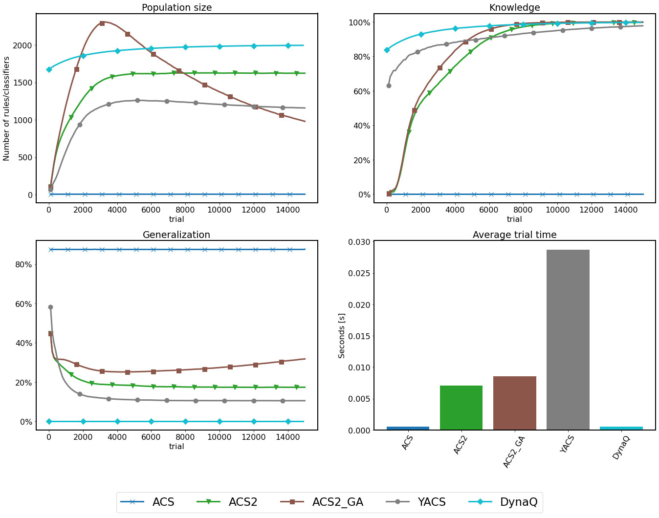
Fig. 3.10 Performance of 3bit rMPX discretized with 10 bins. Metric collected every 100 trials and averaged across 50 independent runs.
Statistical verification
The posterior data distribution was modelled using 50 metric values collected in the last trial and then sampled with 100,000 draws. The obtained results were presented in a table and using the radar plot. The radar plot axes were scaled accordingly, highlighting the relative differences between algorithms.
agents = ['acs', 'acs2', 'acs2_ga', 'yacs', 'dynaq']


def build_models(df: pd.DataFrame, field: str):
    results = {}

    for agent in agents:
        last_trial = df.reset_index(1).query(f'agent == "{agent}"')['trial'].max()
        data_arr = df.query(f'agent == "{agent}" and trial == {last_trial}')[field].to_numpy()
        bayes_model = bayes_estimate(data_arr)
        results[agent] = bayes_model['mu']

    return results


@get_from_cache_or_run(cache_path=f'{cache_dir}/rmpx_3bit/bayes/population.dill')
def build_population_model(df: pd.DataFrame):
    return build_models(df, 'population')


@get_from_cache_or_run(cache_path=f'{cache_dir}/rmpx_3bit/bayes/knowledge.dill')
def build_knowledge_models(df: pd.DataFrame):
    return build_models(df, 'knowledge')


@get_from_cache_or_run(cache_path=f'{cache_dir}/rmpx_3bit/bayes/generalization.dill')
def build_generalization_models(df: pd.DataFrame):
    return build_models(df, 'generalization')


@get_from_cache_or_run(cache_path=f'{cache_dir}/rmpx_3bit/bayes/timing.dill')
def build_timing_models(df: pd.DataFrame):
    return build_models(df, 'time')


population_models = build_population_model(metrics_df)
knowledge_models = build_knowledge_models(metrics_df)
generalization_models = build_generalization_models(metrics_df)
timing_models = build_timing_models(metrics_df)

# prepare table
print_row = lambda r: f'{round(r.mean(), 3)} ± {round(r.std(), 3)}'

payload_df = []
table_data = []

for agent in agents:
    # prepare data frame for visualization
    payload_df.append({
        'agent': agent,
        'knowledge': knowledge_models[agent].mean(),
        'generalization': generalization_models[agent].mean(),
        'population': population_models[agent].mean(),
        'time': timing_models[agent].mean()
    })

    # add data to table
    table_data.append([agent.upper(),
                       print_row(knowledge_models[agent]),
                       print_row(generalization_models[agent]),
                       print_row(population_models[agent]),
                       print_row(timing_models[agent])])

rmpx_bayes_df = pd.DataFrame(payload_df).set_index('agent')

bayes_table = tabulate(table_data,
                       headers=['', 'Knowledge', 'Generalization', 'Population', 'Trial time'],
                       tablefmt="html", stralign='right')

glue('ch33_1_bayes_table', HTML(bayes_table), display=False)
glue('ch33_1_bayes_fig', plot_bayes_comparison(rmpx_bayes_df, 'rMPX', agents, plot_filename=f'{plot_dir}/rmpx_3bit_bayes.png'), display=False)
Knowledge Generalization Population Trial time ACS 0.0 ± 0.0 0.875 ± 0.001 4.0 ± 0.001 0.001 ± 0.001 ACS2 0.998 ± 0.001 0.174 ± 0.001 1622.405 ± 7.313 0.007 ± 0.001 ACS2_GA 1.0 ± 0.001 0.318 ± 0.001 977.517 ± 5.966 0.006 ± 0.001 YACS 0.978 ± 0.001 0.106 ± 0.005 1160.178 ± 6.192 0.03 ± 0.001 DYNAQ 0.998 ± 0.001 0.0 ± 0.0 2000.0 ± 0.001 0.0 ± 0.0
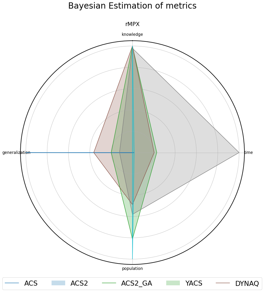
Fig. 3.11 Normalized metrics presented on the radar plot for the 3bit rMPX environment.
Observations
The examined problem input space size is \(2\cdot 10^3=2000\) individual states. Even though using the excessive-resolution size, almost every algorithm built the internal model of the environment in an imposed number of trials.
ACS
Only the ACS agent could not go beyond four semi-general classifiers in the whole experiment, being incapable of learning any of the transitions. Therefore, the generalization and trial-time metrics cannot be directly compared to other agents due to the wrong population size.
ACS2
The successor of ACS - ACS2 ultimately learned the environment using significantly fewer classifiers than the problem input size. The GA extension has a positive effect on compacting the population size and increasing generalization.
YACS
The heuristic nature of YACS allows it to gain knowledge at the beginning of the experiment rapidly. However, the lack of generalization capabilities provides the worst generalization compared to both ACS2 variants. Moreover, the trial execution time is significantly larger than in other systems because all visited states are represented and processed inside the agent’s memory.
Dyna-Q
By design, the Dyna-Q algorithm does not expose any generalization capabilities - therefore is unable to learn latently with more compacted knowledge representation. Due to the lookahead capabilities, the system rapidly learned all available transitions while operating faster than competitors.
Software packages used
import session_info

session_info.show()
Click to view session information
-----
bitstring           3.1.7
gym                 0.21.0
gym_multiplexer     NA
lcs                 NA
matplotlib          3.5.1
myst_nb             0.13.1
numpy               1.22.1
pandas              1.4.0
session_info        1.0.0
src                 (embedded book's utils module)
tabulate            0.8.9
-----
Click to view modules imported as dependencies
PIL                         8.4.0
arviz                       0.11.2
asttokens                   NA
attr                        21.4.0
babel                       2.9.1
backcall                    0.2.0
beta_ufunc                  NA
binom_ufunc                 NA
brotli                      NA
cachetools                  5.0.0
certifi                     2021.10.08
cffi                        1.15.0
cftime                      1.5.2
charset_normalizer          2.0.10
click                       7.1.2
cloudpickle                 2.0.0
colorama                    0.4.4
colorful                    0.5.4
colorful_orig               0.5.4
cryptography                36.0.1
cycler                      0.10.0
cython_runtime              NA
databricks_cli              NA
dateutil                    2.8.2
debugpy                     1.5.1
decorator                   5.1.1
defusedxml                  0.7.1
dill                        0.3.4
docutils                    0.16
entrypoints                 0.3
executing                   0.8.2
fastprogress                0.2.7
filelock                    3.4.2
google                      NA
greenlet                    1.1.2
grpc                        1.43.0
hiredis                     2.0.0
idna                        3.3
imagesize                   NA
importlib_metadata          NA
ipykernel                   6.7.0
ipython_genutils            0.2.0
ipywidgets                  7.6.5
jedi                        0.18.1
jinja2                      3.0.3
jsonschema                  3.2.0
jupyter_cache               0.4.3
jupyter_sphinx              0.3.2
jupyterlab_pygments         0.1.2
kiwisolver                  1.3.2
linkify_it                  1.0.3
markdown_it                 1.1.0
markupsafe                  2.0.1
matplotlib_inline           NA
mdit_py_plugins             0.2.8
mistune                     0.8.4
mlflow                      1.23.1
mpl_toolkits                NA
msgpack                     1.0.3
myst_parser                 0.15.2
nbclient                    0.5.10
nbconvert                   6.4.1
nbformat                    5.1.3
nbinom_ufunc                NA
netCDF4                     1.5.8
packaging                   21.3
pandocfilters               NA
parso                       0.8.3
pexpect                     4.8.0
pickleshare                 0.7.5
pkg_resources               NA
prompt_toolkit              3.0.26
psutil                      5.9.0
ptyprocess                  0.7.0
pure_eval                   0.2.2
pvectorc                    NA
pydev_ipython               NA
pydevconsole                NA
pydevd                      2.6.0
pydevd_concurrency_analyser NA
pydevd_file_utils           NA
pydevd_plugins              NA
pydevd_tracing              NA
pygments                    2.11.2
pylab                       NA
pymc3                       3.11.4
pyparsing                   3.0.7
pyrsistent                  NA
pytz                        2021.3
ray                         1.9.2
redis                       4.1.2
requests                    2.27.1
scipy                       1.7.3
semver                      2.13.0
setproctitle                1.2.2
setuptools                  60.5.0
six                         1.16.0
socks                       1.7.1
sphinx                      4.4.0
sphinxcontrib               NA
sqlalchemy                  1.4.31
stack_data                  0.1.4
testpath                    0.5.0
theano                      1.1.2
tornado                     6.1
tqdm                        4.62.3
traitlets                   5.1.1
typing_extensions           NA
uc_micro                    1.0.1
unicodedata2                NA
urllib3                     1.26.8
wcwidth                     0.2.5
xarray                      0.21.0
yaml                        6.0
zipp                        NA
zmq                         22.3.0
-----
IPython             8.0.1
jupyter_client      7.1.2
jupyter_core        4.9.1
notebook            6.4.8
-----
Python 3.9.10 | packaged by conda-forge | (main, Feb  1 2022, 21:24:11) [GCC 9.4.0]
Linux-5.13.0-30-generic-x86_64-with-glibc2.31
-----
Session information updated at 2022-02-24 12:35