Experiment 2 - Nature of the intervals
Contents
import pathlib
from typing import List

import gym
import gym_checkerboard  # noqa: F401
import lcs.agents.racs as racs
import matplotlib.pyplot as plt
import numpy as np
import pandas as pd
from lcs.agents.racs.metrics import count_averaged_regions
from lcs.metrics import population_metrics
from lcs.representations.RealValueEncoder import RealValueEncoder

from myst_nb import glue

from IPython.display import display, HTML
from tabulate import tabulate

from src.bayes_estimation import bayes_estimate
from src.commons import NUM_EXPERIMENTS
from src.decorators import repeat, get_from_cache_or_run
from src.utils import build_plots_dir_path, build_cache_dir_path
from src.visualization import PLOT_DPI

plt.ioff()  # turn off interactive plotting

root_dir = pathlib.Path().cwd().parent.parent.parent.parent
cwd_dir = pathlib.Path().cwd()

plot_dir = build_plots_dir_path(root_dir) / cwd_dir.parent.name / cwd_dir.name
cache_dir = build_cache_dir_path(root_dir) / cwd_dir.parent.name / cwd_dir.name

TRIALS = 15_000
USE_RAY = True

def encode(p, bits):
    return int(RealValueEncoder(bits).encode(p))


def metrics_to_df(metrics: List) -> pd.DataFrame:
    lst = [[
        d['trial'],
        d['population'],
        d['reliable'],
        d['reward'],
        d['regions'][1],
        d['regions'][2],
        d['regions'][3],
        d['regions'][4],
    ] for d in metrics]

    df = pd.DataFrame(lst, columns=['trial', 'population', 'reliable', 'reward', 'region_1', 'region_2', 'region_3', 'region_4'])
    df = df.set_index('trial')
    df['phase'] = df.index.map(lambda t: "explore" if t % 2 == 0 else "exploit")

    return df


def average_experiment_runs(runs_dfs: List[pd.DataFrame]) -> pd.DataFrame:
    return pd.concat(runs_dfs).groupby(['trial', 'phase']).mean().reset_index(level='phase')


def single_experiment(env_provider, encoder_bits, trials):
    env = env_provider()
    env.reset()

    def _metrics(agent, environment):
        population = agent.population
        metrics = {
            'regions': count_averaged_regions(population)
        }

        # Add basic population metrics
        metrics.update(population_metrics(population, environment))
        return metrics

    cfg = racs.Configuration(
        classifier_length=env.observation_space.shape[0],
        number_of_possible_actions=env.action_space.n,
        encoder=RealValueEncoder(encoder_bits),
        user_metrics_collector_fcn=_metrics,
        epsilon=0.9,
        do_ga=True,
        theta_r=0.9,
        theta_i=0.3,
        theta_ga=100,
        cover_noise=0.1,
        mutation_noise=0.25,
        chi=0.6,
        mu=0.2)

    # create agent
    agent = racs.RACS(cfg)

    # run computations
    metrics = agent.explore_exploit(env, trials)

    return metrics_to_df(metrics)


def plot_condition_interval_regions(df, window=10, plot_filename=None):
    fig, ax = plt.subplots(figsize=(15, 7))

    df['region_1'].rolling(window=window).mean().plot(label='Region 1 [pi, qi)', ax=ax)
    df['region_2'].rolling(window=window).mean().plot(label='Region 2 [pmin, qi)', ax=ax)
    df['region_3'].rolling(window=window).mean().plot(label='Region 3 [pi, qmax)', ax=ax)
    df['region_4'].rolling(window=window).mean().plot(label='Region 4 [pmin, qmax)', ax=ax)

    ax.set_title('Condition Interval Regions')
    ax.set_xlabel('Trial')
    ax.set_ylabel('Proportion')
    plt.legend()

    if plot_filename:
        fig.savefig(plot_filename, dpi=PLOT_DPI, bbox_inches='tight')

    return fig


def plot_population(df, window=10, plot_filename=None):
    fig, ax = plt.subplots(figsize=(15, 7))

    df['population'].rolling(window=window).mean().plot(label='macroclassifiers', ax=ax)
    df['reliable'].rolling(window=window).mean().plot(label='reliable', ax=ax)

    ax.set_title('Classifier numerosity')
    ax.set_xlabel('Trial')
    ax.set_ylabel('Number of classifiers')
    ax.set_yscale('log')
    plt.legend()

    if plot_filename:
        fig.savefig(plot_filename, dpi=PLOT_DPI, bbox_inches='tight')

    return fig


def plot_performance(df, window=50, plot_filename=None):
    fig, ax = plt.subplots(figsize=(15, 7))

    explore_df = df[df['phase'] == 'explore']
    exploit_df = df[df['phase'] == 'exploit']

    explore_df['reward'].rolling(window=window).mean().plot(label='explore', ax=ax)
    exploit_df['reward'].rolling(window=window).mean().plot(label='exploit', ax=ax)
    plt.axhline(1.0, c='black', linestyle=':')

    ax.set_title('Performance (average reward)')
    ax.set_xlabel('Trial')
    ax.set_ylabel('Reward')
    ax.set_ylim([.4, 1.05])
    plt.legend()

    if plot_filename:
        fig.savefig(plot_filename, dpi=PLOT_DPI, bbox_inches='tight')

    return fig

def encode_array(arr, bits):
    return np.fromiter((encode(x, bits=bits) for x in arr), int)

def plot_checkerboard_splits(splits, bits, points=100, plot_filename=None):
    fig = plt.figure(figsize=(12, 5))
    ax = fig.add_subplot(111)

    # Visualize splits
    for k in np.linspace(0, 1, splits + 1):
        ax.axvline(x=k, ymin=0, ymax=1, linewidth=1, linestyle=':', color='black')

    # Add some points
    x = np.random.random(points)
    y = np.random.random(points)
    colors = encode_array(x, bits)
    ax.scatter(x, y, c=colors, s=20, alpha=.8)

    for i, txt in enumerate(colors):
        ax.annotate(txt, xy=(x[i] + .005, y[i] + .005), size=8, alpha=.8)

    ax.set_title(f"{bits}-bit encoder mapping on {splits} checkerboard splits")
    ax.set_xlabel("Perception value")
    ax.set_ylim(-0.1, 1.1)
    ax.set_xlim(-0.02, 1.02)
    ax.get_yaxis().set_visible(False)

    if plot_filename:
        fig.savefig(plot_filename, dpi=PLOT_DPI)

    return fig

glue('32_e2_trials', TRIALS, display=False)
glue('32_e2_checkerboard_3_splits_4_bits_fig', plot_checkerboard_splits(splits=3, bits=4, plot_filename=f'{plot_dir}/checkerboard_3_splits_4_bits.png'), display=False)
Experiment 2 - Nature of the intervals
In order to provide the correct answer to the checkerboard problem, the agent must be able to correctly partition the hyper-rectangular solution space. Four categories are used to determine the nature of the evolved condition intervals:
Region 1 \([p_i, q_i]\) - consists of specific intervals.
Region 2 \([p_{min}, q_i)\) - interval bounded from the right side.
Region 3 \([p_i, q_{max})\) - interval bounded from the left side.
Region 4 \([p_{min}, q_{max})\) - general interval (“don’t care”).
The two-dimensional checkerboard divided by three splits in each direction is used. The experiment uses the rACS agent and evaluates its performance with different encoding values. Because of the splits, the system response is dependent on precise boundaries estimations. Figure 3.6 shows possible ambiguities near the split lines, where the same nominal value is applicable in both regions.
As in the previous section, in each trial of the experiment, the agent alternates between explore and exploit phases for the total of 15000 trials. Each independent pass is averaged across 50 times. For the collected metrics, besides the average performance and the population size, the proportion of condition interval regions is collected for each trial.
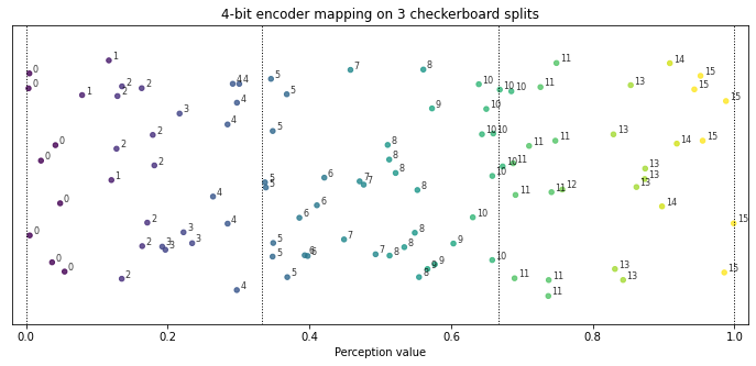
Fig. 3.6 Example of dividing the space into three equal splits. When using low encoding resolution potential ambiguity is visible near the splitting lines.
Results
Figures 3.7, 3.8 and 3.9 illustrate the metrics progression on the 3x3 Checkerboard problem using 4 bit interval encoding. Due to brevity the plots for other encoding values were not presented, but final values are outlined using statistical estimation.
rACS parameters
\(\beta=0.05\), \(\gamma = 0.95\), \(\theta_r = 0.9\), \(\theta_i=0.3\), \(\epsilon = 0.9\), \(\theta_{GA} = 100\), \(m_u=0.2\), \(\chi=0.6\), \(\epsilon_{cover} = 0.1\), \(\epsilon_{mutation}=0.25\).
def checkboard_env_provider():
    import gym_checkerboard  # noqa: F401
    return gym.make('checkerboard-2D-3div-v0')

@get_from_cache_or_run(cache_path=f'{cache_dir}/checkerboard_3x3/encoding_1bit.dill')
@repeat(num_times=NUM_EXPERIMENTS, use_ray=USE_RAY)
def run_checkerboard_1bit_encoding():
    return single_experiment(checkboard_env_provider, encoder_bits=1, trials=TRIALS)

@get_from_cache_or_run(cache_path=f'{cache_dir}/checkerboard_3x3/encoding_2bit.dill')
@repeat(num_times=NUM_EXPERIMENTS, use_ray=USE_RAY)
def run_checkerboard_2bit_encoding():
    return single_experiment(checkboard_env_provider, encoder_bits=2, trials=TRIALS)

@get_from_cache_or_run(cache_path=f'{cache_dir}/checkerboard_3x3/encoding_3bit.dill')
@repeat(num_times=NUM_EXPERIMENTS, use_ray=USE_RAY)
def run_checkerboard_3bit_encoding():
    return single_experiment(checkboard_env_provider, encoder_bits=3, trials=TRIALS)

@get_from_cache_or_run(cache_path=f'{cache_dir}/checkerboard_3x3/encoding_4bit.dill')
@repeat(num_times=NUM_EXPERIMENTS, use_ray=USE_RAY)
def run_checkerboard_4bit_encoding():
    return single_experiment(checkboard_env_provider, encoder_bits=4, trials=TRIALS)

@get_from_cache_or_run(cache_path=f'{cache_dir}/checkerboard_3x3/encoding_5bit.dill')
@repeat(num_times=NUM_EXPERIMENTS, use_ray=USE_RAY)
def run_checkerboard_5bit_encoding():
    return single_experiment(checkboard_env_provider, encoder_bits=5, trials=TRIALS)

# run computations
checkerboard_encoding_1bit_runs = run_checkerboard_1bit_encoding()
checkerboard_encoding_2bit_runs = run_checkerboard_2bit_encoding()
checkerboard_encoding_3bit_runs = run_checkerboard_3bit_encoding()
checkerboard_encoding_4bit_runs = run_checkerboard_4bit_encoding()
checkerboard_encoding_5bit_runs = run_checkerboard_5bit_encoding()

# average runs
checkerboard_encoding_4bit_avg = average_experiment_runs(checkerboard_encoding_4bit_runs)

# generate plots
glue('checkerboard4bit-enc4bit-regions-fig', plot_condition_interval_regions(checkerboard_encoding_4bit_avg, plot_filename=f'{plot_dir}/checkerboard_4bit_regions.png'), display=False)
glue('checkerboard4bit-enc4bit-performance-fig', plot_performance(checkerboard_encoding_4bit_avg, plot_filename=f'{plot_dir}/checkerboard_4bit_performance.png'), display=False)
glue('checkerboard4bit-enc4bit-population-fig', plot_population(checkerboard_encoding_4bit_avg, plot_filename=f'{plot_dir}/checkerboard_4bit_population.png'), display=False)
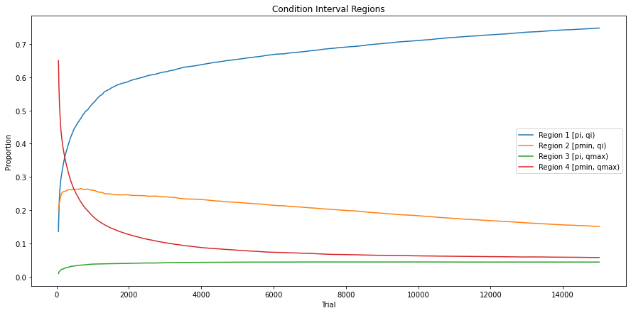
Fig. 3.7 Evolution of condition interval regions in 3x3 Checkerboard environment encoded with 4 bits.
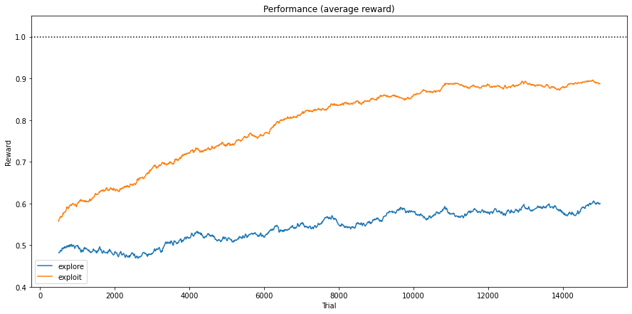
Fig. 3.8 Average reward obtained in 3x3 Checkerboard environment encoded with 4 bits.
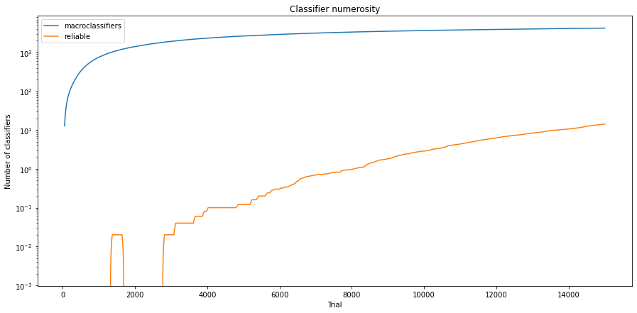
Fig. 3.9 Population size of 3x3 Checkerboard environment encoded with 4 bits (notice the logarithmic scalling of y-axis).
Statistical verification
To statistically assess the population size and region ratios, the posterior data distribution was modelled using 50 metric values collected in the last trial and then sampled with 100,000 draws. For the obtained reward, the mean value from the last 100 exploit trials is considered as a representative state of algorithm performance.
def build_models(dfs: List[pd.DataFrame], field: str):
    query_condition = f'trial == {TRIALS}'  # last trial
    results = []
    for df in dfs:
        data_arr = df.query(query_condition)[field].to_numpy()
        bayes_model = bayes_estimate(data_arr)
        results.append((bayes_model['mu'], bayes_model['std']))

    return results

def get_average_reward(dfs: List[pd.DataFrame], last_n_runs: int = 100):
    results = []
    for df in dfs:
        avg_reward = df.query('phase == "exploit"').groupby('trial').mean().iloc[-last_n_runs:]['reward'].mean()
        results.append(avg_reward)
    return results

@get_from_cache_or_run(cache_path=f'{cache_dir}/checkerboard_3x3/bayes/region_1.dill')
def build_region_1_models(dfs: List[pd.DataFrame]):
    return build_models(dfs, 'region_1')

@get_from_cache_or_run(cache_path=f'{cache_dir}/checkerboard_3x3/bayes/region_2.dill')
def build_region_2_models(dfs: List[pd.DataFrame]):
    return build_models(dfs, 'region_2')

@get_from_cache_or_run(cache_path=f'{cache_dir}/checkerboard_3x3/bayes/region_3.dill')
def build_region_3_models(dfs: List[pd.DataFrame]):
    return build_models(dfs, 'region_3')

@get_from_cache_or_run(cache_path=f'{cache_dir}/checkerboard_3x3/bayes/region_4.dill')
def build_region_4_models(dfs: List[pd.DataFrame]):
    return build_models(dfs, 'region_4')

@get_from_cache_or_run(cache_path=f'{cache_dir}/checkerboard_3x3/bayes/population.dill')
def build_population_models(dfs: List[pd.DataFrame]):
    return build_models(dfs, 'population')

@get_from_cache_or_run(cache_path=f'{cache_dir}/checkerboard_3x3/bayes/reliable.dill')
def build_reliable_models(dfs: List[pd.DataFrame]):
    return build_models(dfs, 'reliable')

bayes_results_dfs = [
    pd.concat(checkerboard_encoding_1bit_runs),
    pd.concat(checkerboard_encoding_2bit_runs),
    pd.concat(checkerboard_encoding_3bit_runs),
    pd.concat(checkerboard_encoding_4bit_runs),
    pd.concat(checkerboard_encoding_5bit_runs),
]

region_1_models = build_region_1_models(bayes_results_dfs)
region_2_models = build_region_2_models(bayes_results_dfs)
region_3_models = build_region_3_models(bayes_results_dfs)
region_4_models = build_region_4_models(bayes_results_dfs)
population_models = build_population_models(bayes_results_dfs)
reliable_models = build_reliable_models(bayes_results_dfs)
avg_rewards = get_average_reward(bayes_results_dfs)

bayes_table_data = [
    ['Region 1'] + [f'{round(r[0].mean(), 2)} ± {round(r[0].std(), 2)}' for r in region_1_models],
    ['Region 2'] + [f'{round(r[0].mean(), 2)} ± {round(r[0].std(), 2)}' for r in region_2_models],
    ['Region 3'] + [f'{round(r[0].mean(), 2)} ± {round(r[0].std(), 2)}' for r in region_3_models],
    ['Region 4'] + [f'{round(r[0].mean(), 2)} ± {round(r[0].std(), 2)}' for r in region_4_models],
    ['population of classifiers'] + [f'{round(r[0].mean(), 2)} ± {round(r[0].std(), 2)}' for r in population_models],
    ['reliable classifiers'] + [f'{round(r[0].mean(), 2)} ± {round(r[0].std(), 2)}' for r in reliable_models],
    ['reward from last 100 exploit runs'] + [f'{round(r, 2)}' for r in avg_rewards],
]

table = tabulate(bayes_table_data, headers=['', '1 bit', '2 bit', '3 bit', '4 bit', '5 bit'], tablefmt="html", stralign='right')
display(HTML(table))
| 1 bit | 2 bit | 3 bit | 4 bit | 5 bit | |
|---|---|---|---|---|---|
| Region 1 | 0.0 ± 0.0 | 0.32 ± 0.0 | 0.69 ± 0.0 | 0.75 ± 0.0 | 0.71 ± 0.0 |
| Region 2 | 0.46 ± 0.0 | 0.35 ± 0.0 | 0.18 ± 0.0 | 0.15 ± 0.0 | 0.2 ± 0.0 |
| Region 3 | 0.26 ± 0.01 | 0.14 ± 0.0 | 0.08 ± 0.0 | 0.04 ± 0.0 | 0.02 ± 0.0 |
| Region 4 | 0.27 ± 0.01 | 0.19 ± 0.0 | 0.05 ± 0.0 | 0.06 ± 0.0 | 0.08 ± 0.0 |
| population of classifiers | 20.22 ± 0.38 | 52.63 ± 0.57 | 735.64 ± 8.67 | 4244.18 ± 35.75 | 10358.61 ± 47.0 |
| reliable classifiers | -0.0 ± 0.0 | 8.0 ± 0.0 | 89.51 ± 1.17 | 14.42 ± 0.6 | 0.64 ± 0.16 |
| reward from last 100 exploit runs | 0.52 | 0.71 | 0.81 | 0.89 | 0.78 |
Observations
In most experiments, the rACS agent builds the population consisting primarily of Region 1 interval predicates. The amount of attributes represented as Region 3 and 4, spanning to the maximum value from the right side, tends to diminish. However, the results are correlated with the number of trials that were kept the same in all cases. More precise boundary representation naturally would require more trials to converge. However, for the first four bits, there is the following trend can be noticed when intensifying encoding resolution:
Ratio of Region 1 attributes increases,
Ratio of Region 2, 3, 4 attributes decreases.
This is caused by the lack of online rule compaction or consolidation mechanism. The only possibility for the agent to create a more general attribute is due to the mutation algorithm controlled by the \(\epsilon_{mutation}\) parameter. However, this value must be set carefully because limitations of selected encoding resolution can inadvertently ignore its effect.
The other metrics also show the hypothesis about the need for more trials. The size of the overall population is correlated with the number of encoding bits, but it became more difficult for the agent to discriminate between reliable classifiers. For example, when using 5-bits encoding after 15000 trials, there is no single reliable classifier despite having a population with more than 10 thousand individuals.
The experiment with 1-bit encoding also confirms the situation when it is impossible to learn the environment with hyper-plane decision boundary successfully. Such representation is insufficient to handle regularities, resulting in unreliable classifiers and random average rewards from exploit runs.
Software packages used
import session_info

session_info.show()
Click to view session information
-----
gym                 0.21.0
gym_checkerboard    NA
lcs                 NA
matplotlib          3.5.1
myst_nb             0.13.1
numpy               1.22.1
pandas              1.4.0
session_info        1.0.0
src                 (embedded book's utils module)
tabulate            0.8.9
-----
Click to view modules imported as dependencies
PIL                         8.4.0
arviz                       0.11.2
asttokens                   NA
attr                        21.4.0
babel                       2.9.1
backcall                    0.2.0
beta_ufunc                  NA
binom_ufunc                 NA
brotli                      NA
cachetools                  5.0.0
certifi                     2021.10.08
cffi                        1.15.0
cftime                      1.5.2
charset_normalizer          2.0.10
click                       7.1.2
cloudpickle                 2.0.0
colorama                    0.4.4
colorful                    0.5.4
colorful_orig               0.5.4
cryptography                36.0.1
cycler                      0.10.0
cython_runtime              NA
databricks_cli              NA
dataslots                   NA
dateutil                    2.8.2
debugpy                     1.5.1
decorator                   5.1.1
defusedxml                  0.7.1
dill                        0.3.4
docutils                    0.16
entrypoints                 0.3
executing                   0.8.2
fastprogress                0.2.7
filelock                    3.4.2
google                      NA
greenlet                    1.1.2
grpc                        1.43.0
hiredis                     2.0.0
idna                        3.3
imagesize                   NA
importlib_metadata          NA
ipykernel                   6.7.0
ipython_genutils            0.2.0
ipywidgets                  7.6.5
jedi                        0.18.1
jinja2                      3.0.3
jsonschema                  3.2.0
jupyter_cache               0.4.3
jupyter_sphinx              0.3.2
jupyterlab_pygments         0.1.2
kiwisolver                  1.3.2
linkify_it                  1.0.3
markdown_it                 1.1.0
markupsafe                  2.0.1
matplotlib_inline           NA
mdit_py_plugins             0.2.8
mistune                     0.8.4
mlflow                      1.23.1
mpl_toolkits                NA
msgpack                     1.0.3
myst_parser                 0.15.2
nbclient                    0.5.10
nbconvert                   6.4.1
nbformat                    5.1.3
nbinom_ufunc                NA
netCDF4                     1.5.8
packaging                   21.3
pandocfilters               NA
parso                       0.8.3
pexpect                     4.8.0
pickleshare                 0.7.5
pkg_resources               NA
prompt_toolkit              3.0.26
psutil                      5.9.0
ptyprocess                  0.7.0
pure_eval                   0.2.2
pvectorc                    NA
pydev_ipython               NA
pydevconsole                NA
pydevd                      2.6.0
pydevd_concurrency_analyser NA
pydevd_file_utils           NA
pydevd_plugins              NA
pydevd_tracing              NA
pygments                    2.11.2
pylab                       NA
pymc3                       3.11.4
pyparsing                   3.0.7
pyrsistent                  NA
pytz                        2021.3
ray                         1.9.2
redis                       4.1.2
requests                    2.27.1
scipy                       1.7.3
semver                      2.13.0
setproctitle                1.2.2
setuptools                  60.5.0
six                         1.16.0
socks                       1.7.1
sphinx                      4.4.0
sphinxcontrib               NA
sqlalchemy                  1.4.31
stack_data                  0.1.4
testpath                    0.5.0
theano                      1.1.2
tornado                     6.1
tqdm                        4.62.3
traitlets                   5.1.1
typing_extensions           NA
uc_micro                    1.0.1
unicodedata2                NA
urllib3                     1.26.8
wcwidth                     0.2.5
xarray                      0.21.0
yaml                        6.0
zipp                        NA
zmq                         22.3.0
-----
IPython             8.0.1
jupyter_client      7.1.2
jupyter_core        4.9.1
notebook            6.4.8
-----
Python 3.9.10 | packaged by conda-forge | (main, Feb  1 2022, 21:24:11) [GCC 9.4.0]
Linux-5.13.0-30-generic-x86_64-with-glibc2.31
-----
Session information updated at 2022-03-06 14:30