Real-valued input challenge
Contents
2.2. Real-valued input challenge
Most real-world environments or datasets are represented using exclusively continue-valued inputs or alongside discrete attributes. Unfortunately, the described ALCS implementations were not initially designed for such representations. The fundamental modification required to overcome the limitation above is the adaptation of rule representation within the system. Despite the variety of possible approaches listed in this chapter, each comes with its own merits and perils.
Two significant concepts involving the discretization and interval encoding using dedicated alphabets will be pursued later, while the hindmost ones involving the neural network and fuzzy logic will be only mentioned. There are two main reasons for this decision:
drastic changes in rule representation requires significant modifications in existing and tightly coupled components. In some cases, some of them are not usable in their proposed form - like the ALP component in ACS systems needs a complete redefinition for other alphabet encodings,
rule interpretability is relevantly blemished.
Therefore, even if some approaches are more appealing for the problem, their usage violates principal ALCS virtue of transparency (creating a compact set of human-readable rules) or does not formally specify the behaviour of related inner mechanisms fulfilling the evolution and assessing each classifier. However, more detailed research is highly advised but will not be pursued herein.
Discretization
One of the approaches for handling continuous attributes is to partition them into a number of sub-ranges and treat each sub-range as a category. This process is known as discretization and is used across many families of ML algorithms in order to create better models [94]. In the XCS family, the modification of XCSI [95] adopted the algorithm for the integer domain. The modification was evaluated on the Wisconsin Breast Cancer dataset and turned out to be competitive with other ML algorithms. Minding the nature of ALCS, the usage of such nominal values would also be the most straightforward approach. ALCS systems by design are not limited by ternary representation, therefore creating an arbitrary number of potential states is achievable. The first such implementation called rACS was proposed by Unold and Mianowski in 2016 [41] and tested successfully on Corridor and Grid environments. Both have a regular structure, meaning that the intervals are evenly distributed throughout the investigated range.
Unfortunately, the number of ways to discretize a continuous attribute is infinite. Kotsiantis in [96] takes a survey of possible discretization techniques, but in this work, the preferred method is to divide the search-space into \(n\) equally spaced intervals, referred later as bins or buckets. When the \(n\) is large, system precision is increased, resulting obviously in the growth of the classifier population. Such a population can be further optimized by compacting the classifiers operating in the neighbouring space regions [97] [95]. On the contrary, when the \(n\) is low, the system under-performs due to the inability of creating accurate classifiers.
The process of assigning a discrete value for each consecutive interval region within \([0, 1]\) range is depicted on Figure 2.4.
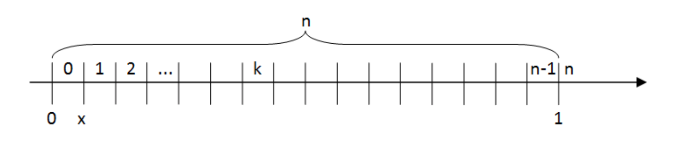
Fig. 2.4 Representation of allele in rACS as a natural number of the partition. Figure taken from [41].
Such a solution for real-value representation in a simple scenario does not require significant changes to any components and retain the human readability and interpretability of created rules. However, when an arbitrary number of bins for each observation attribute is used, certain modifications might be necessary (for example, additional restrictions for the GA cross-over operator).
Interval predicates
The discretization approach assumed that a distinct value of the condition attribute represents a fixed-length interval part of an input range. Another approach is to encode the input using custom hyper-rectangular boundaries described by half-open interval \([p_i, q_i)\), which matches the environment signal \(x_i\) if \(p_i \leq x_i < q_i\).
Such approach facilitates creation of more general and compact population size, due to arbitrarily interval ranges. In 1999 Wilson took the approach to adapt the XCS to automatically search for optimally decisive thresholds [32]. His approach representation named center-spread representation (CSR) used to represent an interval tuple \((c_i, s_i) \ \text{where} \ c_i, s_i \in \mathbb{R}\) where \(c_i\) is the center of the interval, and \(s_i\) its spread. The interval is therefore described in Equation (2.1):
His system, called XCSR, differs only at the input interface, mutation and covering operators. Preliminary tests revealed the weakness of the crude mutation operator. Moreover, the testing environment, which is very regular and therefore did not challenge the agent with interesting problems like noise or data contradiction.
In 2003 Stone and Bull thoroughly addressed those problems in [34] by introducing two new representations - ordered-bounded (OBR) and unordered-bounded (UBR). The OBR is an extension of Wilson XCSI [29] but enhanced with real-valued interval tuple \((l_i, u_i) \ \text{where} \ l_i, u_i \in \mathbb{R}\). Here \(l_i\) and \(u_i\) relates to lower and upper bounds, respectively. The encoding imposes \(l_i < u_i\) ordering; therefore, all system components that might inadvertently change must be recognized and taken care of. This requirement was relaxed in UBR [33], thus the same interval can be encoded by both \((p_i, q_i)\) and \((q_i, p_i)\). The advantage is that no operator constraints are needed when the ordering restriction is violated, which constitutes a form of epistasis between \(l_i\) and \(u_i\), as their values are mutually dependent. The authors showed that CSR and OBR are biased in interval generation in bounded solution spaces. The UBR obviating limitations of OBR was assumed to yield better results in one of the testing problems and therefore considered superior to the other ones.
Finally, in 2005 Dam and Abbass [35] recognized that UBR changes the semantics of the chromosome by alternating between min and max genes. This discrepancy is challenging for the XCS because it disturbs the genetic process evolving the population of classifiers [3] [49]. They present the Min-Percentage representation of \((m_i, k_i) \ \text{where} \ m_i, k_i \in \mathbb{R}\) tuple, where the interval is determined by the Equation (2.2), which compared with UBR did not provide any substantial improvements.
It is also worth mentioning an important, subtly different, family of learning classifier systems handling real-valued input natively by approximating functions. The most popular implementation of XCSF [33] [98] computes the payoff value locally instead of learning its prediction through a gradient-descent type update. The classifier’s condition covers the continuous input by an OBR interval. Enhanced with additional weights vector, updated by regression techniques, the output prediction can be calculated. The classifier structure was further simplified by eliminating the proposed action. Because of the lack of explicit state anticipation capabilities, the function approximation learning classifiers systems are not considered in this work.
Neural networks
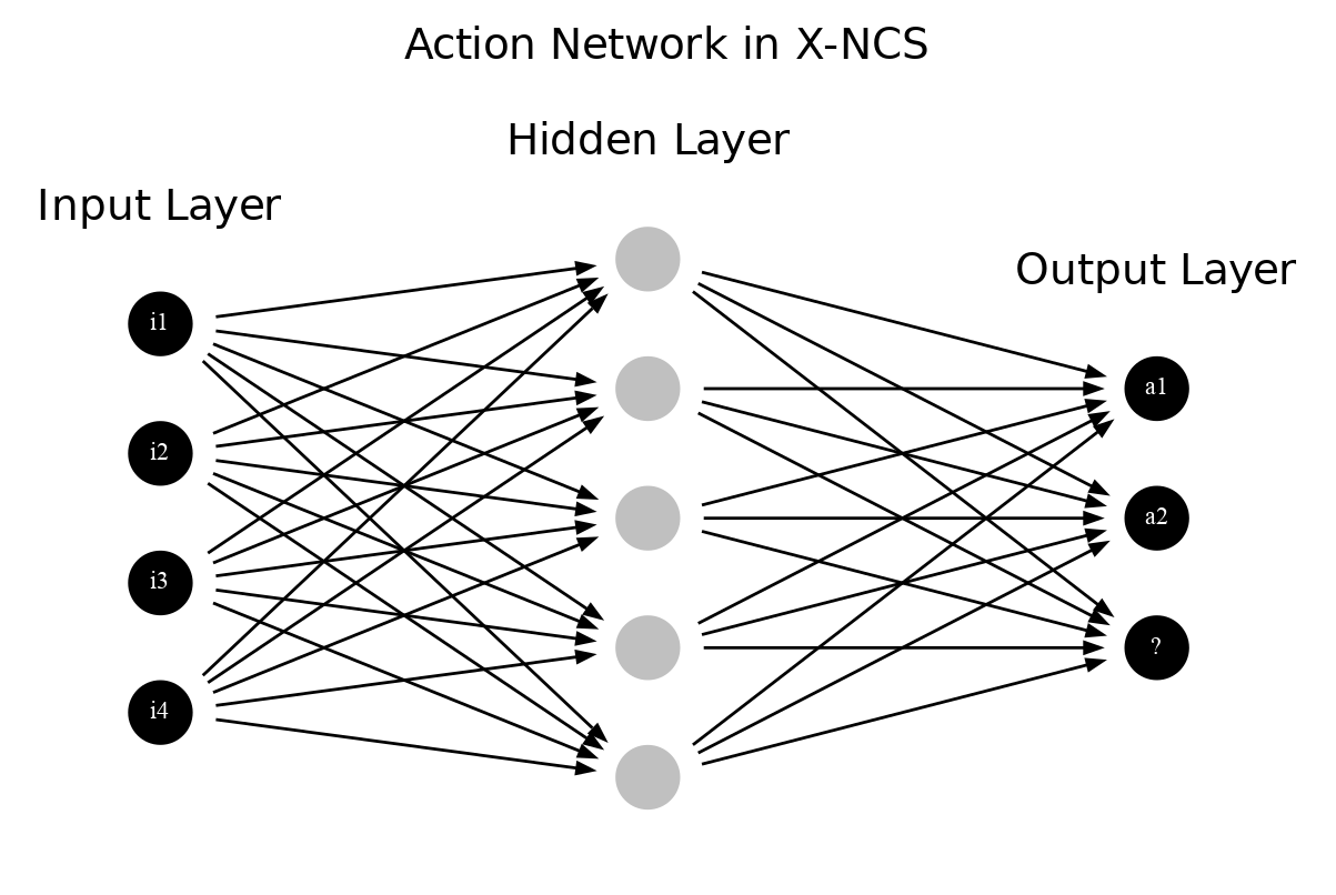
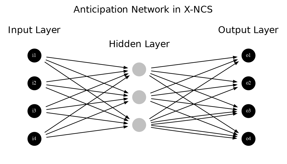
O’Hara and Bull experimented with representing the rule structure of an XCS classifier with two artificial neural networks, introducing the system named X-NCS [99] [100]. While the first one, called the action-network, determines the application condition of the classifiers replacing the condition-action part, the latter one - anticipation network - forms the description of the predicted next state.
Both networks are fully connected multi-layered perceptrons (MLP) with the same nodes in their hidden layer. The input layer in both cases matches the observation state vector provided by the environment. In the action network, the size of an output layer is equal to the number of possible actions incremented with an extra node signifying a non-matching situation. Hence, the anticipation network is responsible for predicting the next state; the size of its output layer is equal to the input one. Figures 2.5 and 2.6 visualize both topologies.
The system starts with an initial random population, containing the maximum number of classifiers considered in a particular experiment, as opposed to standard XCS [30]. The network weights are randomly initialized in the range \([-1.0, 1.0]\) and are updated throughout the experiment using two search techniques - the local search performed by backpropagation complemented by the global sampling performed by GA.
In order to assess the general system error, all of the internal mechanisms remained unchanged except for the calculation of the rule’s absolute error, which is defined as the sum of prediction and lookahead error (measuring the correctness of the prediction).
The critical difference between the classic ternary representation is the lack of explicit wildcard symbol and hence no explicit pass-through of input to anticipations. A concept of a reliable classifier cannot be applied in X-NCS - the anticipation accuracy is based on a percentage of accurate anticipations per presentation.
The authors tested the extension in various configurations showing promising results, especially on discrete multistep problems. Due to novel rule representation, the X-NCS system is suited for real-valued data representation, but the conceptual differences make it difficult to compare it with other systems. Aspects like vague generalization metric, constant population size or the anticipation accuracy computation would require dedicated research solely on this implementation.
Interestingly, two years later, a similar system evolved. The authors take advantage of the idea of both the function mapping [101] and the neural anticipation [100]. The classifier structure was extended with a parametrized anticipatory function \(an_f\), which is trained using supervised learning based on the current state \(\sigma_t\) and the next state \(\sigma_{t+1}\). The proposed XCS with anticipation mappings (XCSAM) system [102] does not use the lookahead error and focuses on the value of actions. The authors claim that the anticipatory capabilities are obtained as the “side effects”. Because of the lack of any dedicated prediction components, the anticipatory burden falls on the function \(an_f\). Preliminary experiments showed that both X-NCS and XCSAM obtain comparable results on discrete multistep environments, however both of the systems can be generalized to problems involving continuous inputs [103].
Fuzzy representation
The Michigan-style genetic fuzzy rule-based system [104] is a machine learning system that employs linguistic rules and fuzzy sets in its representation and an evolutionary algorithm for rule discovery. Casillas proposed relevant modifications to the XCS and introduced a new modification called Fuzzy-XCS [14]. The newly created system was capable of dealing with continuous states and actions while maintaining maximal generalization. A similar solution was also proposed later by Bonarini in [105].
Kondziela undertook an approach to create a fuzzy variant of ACS in 2021 [106]. The presented idea modified the system comprising four major elements [107]:
fuzzification - assigns set membership of current environmental perception,
inference - aggregates the results by comparing the membership functions with collected knowledge,
knowledge-store - stores population of classifiers where representing rules using the Fuzzy Inference System (Mamandi) of
IF..AND..THENstatements [108],defuzzification - provides a single value response obtained from the inference phase determining the final action value.
As the first step the vector of environment signal determines set memberships using predefined functions [109] [105]. Then using the rule representation described by Equation (2.3) the match set is formed. Each input value \(X_i\) is equal to a linguistic set of \(\tilde{A_i} = \{ A_{i1} \lor \dots \lor A_{il} \}\) meaning that classifier internally consists of a rule described with \(\{0, 1, \# \}\) symbols (ternary alphabet).
In the next step, the action set \([A]\) is formed in the same way as in traditional ACS, but the final action selection procedure differs - it is proposed by taking advantage of each rule’s membership function values, and the Center of Gravity method for defuzzification [106].
Preliminary tests made on multistep, discrete maze environments showed that fuzzy ACS implementation successfully predicted more than 75% of encountered situations and maintained a limited number of reliable classifiers (although both metrics were highly oscillating). The author did not report any other operational performance indicators.
The usage of fuzzy logic enables the system to handle the real-valued input naturally. The apparent impediment is the requirement to specify membership functions for each environmental perception upfront. The selection of optimal values is complicated [110], and further increases the number of overall system tunable parameters. The other identified flaw is the GA phase which is not suited for new representation. Both the mutation and cross-over operators should be reviewed accordingly.