Experiment 2 - Deceptive Corridor
Contents
import pathlib
import warnings
from typing import List, Dict

import gym
import gym_fsw  # noqa: F401
import matplotlib.pyplot as plt
import numpy as np
import pandas as pd
from lcs import Perception
from matplotlib.ticker import MultipleLocator, FormatStrFormatter
from myst_nb import glue
from IPython.display import HTML
from tabulate import tabulate
from src.bayes_estimation import bayes_estimate

from src.basic_rl import run_q_learning_alternating, run_r_learning_alternating, qlearning, rlearning
from src.commons import NUM_EXPERIMENTS
from src.decorators import repeat, get_from_cache_or_run
from src.diminishing_reward import common_metrics
from src.observation_wrappers import FSWObservationWrapper
from src.payoff_landscape import get_all_state_action, plot_payoff_landscape
from src.runner import run_experiments_alternating
from src.utils import build_plots_dir_path, build_cache_dir_path
from src.visualization import PLOT_DPI, diminishing_reward_colors

plt.ioff()  # turn off interactive plotting
plt.style.use('../../../src/phd.mplstyle')

root_dir = pathlib.Path().cwd().parent.parent.parent
cwd_dir = pathlib.Path().cwd()

plot_dir = build_plots_dir_path(root_dir) / cwd_dir.name
cache_dir = build_cache_dir_path(root_dir) / cwd_dir.name

def extract_specific_index(runs, env_idx):
    """Selects run metrics for certain environment, ie FSW 40"""
    return [run[env_idx] for run in runs]

def average_experiment_runs(run_df: pd.DataFrame) -> pd.DataFrame:
    return run_df.groupby(['agent', 'trial', 'phase']).mean().reset_index(level='phase')

def plot_pop_and_rho(df, trials, plot_filename=None):
    colors = diminishing_reward_colors()

    expl_df = df[df['phase'] == 'exploit']

    xmax = trials/2

    fig, axs = plt.subplots(2, 1, figsize=(18, 16))

    # Steps in trial plot
    for alg in ['ACS2', 'AACS2_v1', 'AACS2_v2', 'Q-Learning', 'R-Learning']:
        alg_df = expl_df.loc[alg]
        idx = pd.Index(name='exploit trial', data=np.arange(1, len(alg_df) + 1))
        alg_df.set_index(idx, inplace=True)

        alg_df['steps_in_trial'].rolling(window=10).mean().plot(ax=axs[0], label=alg, linewidth=2, color=colors[alg])

    axs[0].set_xlabel("Exploit trial")
    axs[0].set_xlim(1, 500)
    axs[0].xaxis.set_major_locator(MultipleLocator(50))
    axs[0].xaxis.set_minor_locator(MultipleLocator(10))
    axs[0].xaxis.set_major_formatter(FormatStrFormatter('%1.0f'))
    axs[0].xaxis.set_tick_params(which='major', size=10, width=2, direction='in')
    axs[0].xaxis.set_tick_params(which='minor', size=5, width=1, direction='in')

    axs[0].set_ylabel("Number of steps")
    axs[0].yaxis.set_major_locator(MultipleLocator(1))
    axs[0].yaxis.set_tick_params(which='major', size=10, width=2, direction='in')
    axs[0].yaxis.set_tick_params(which='minor', size=5, width=1, direction='in')

    axs[0].set_title('Steps in trial')
    axs[0].legend(loc='upper right', frameon=False)

    # Rho plot
    for alg in ['AACS2_v1', 'AACS2_v2', 'R-Learning']:
        alg_df = expl_df.loc[alg]
        idx = pd.Index(name='exploit trial', data=np.arange(1, len(alg_df) + 1))
        alg_df.set_index(idx, inplace=True)

        alg_df['rho'].plot(ax=axs[1], label=alg, linewidth=2, color=colors[alg])

    axs[1].set_xlim(0, xmax)
    axs[1].set_xlabel("Exploit trial")
    axs[1].xaxis.set_major_locator(MultipleLocator(500))
    axs[1].xaxis.set_minor_locator(MultipleLocator(100))
    axs[1].xaxis.set_major_formatter(FormatStrFormatter('%1.0f'))
    axs[1].xaxis.set_tick_params(which='major', size=10, width=2, direction='in')
    axs[1].xaxis.set_tick_params(which='minor', size=5, width=1, direction='in')

    axs[1].set_ylabel(r"$\mathregular{\rho}$")
    axs[1].yaxis.set_major_locator(MultipleLocator(2))
    axs[1].yaxis.set_minor_locator(MultipleLocator(1))
    axs[1].yaxis.set_tick_params(which='major', size=10, width=2, direction='in')
    axs[1].yaxis.set_tick_params(which='minor', size=5, width=1, direction='in')
    axs[1].set_ylim(0, 11)

    axs[1].set_title(r'Estimated average $\mathregular{\rho}$')

    if plot_filename:
            fig.savefig(plot_filename, dpi=PLOT_DPI, bbox_inches='tight')

    return fig

# settings
trials = 10_000
USE_RAY= True

learning_rate = 0.5
discount_factor = 0.95
epsilon = 0.1
zeta = 0.0001

glue('51-e2-trials', trials, display=False)
Experiment 2 - Deceptive Corridor
Finite State World differentiate from the Corridor by the presence of futile movement available in every step. Moreover, this action alternates between the states, demanding the agent to discriminate between relevant perceptions.
Agent’s behaviour is expected to properly distribute reward across all valuable states, meanwhile ignoring the rest of them. The analysis was performed by executing consecutive 10000 trials alternating between explore and exploit phases. Similarly, as in the previous experiment, there is only one state-observed; thus, the ACS2 genetic generalization mechanism remains turned off.
def fsw10_env_provider():
    import gym_fsw  # noqa: F401
    return FSWObservationWrapper(gym.make(f'fsw-10-v0'))

def fsw20_env_provider():
    import gym_fsw  # noqa: F401
    return FSWObservationWrapper(gym.make(f'fsw-20-v0'))

def fsw40_env_provider():
    import gym_fsw  # noqa: F401
    return FSWObservationWrapper(gym.make(f'fsw-40-v0'))

# Set ACS2/AACS2 configuration parameter dictionary
basic_cfg = {
    'perception_bits': 1,
    'possible_actions': 2,
    'do_ga': False,
    'beta': learning_rate,
    'epsilon': epsilon,
    'gamma': discount_factor,
    'zeta': zeta,
    'user_metrics_collector_fcn': common_metrics,
    'biased_exploration_prob': 0,
    'metrics_trial_freq': 1
}


def run_multiple_qlearning(env_provider):
    fsw_env = env_provider()
    init_Q = np.zeros((fsw_env.observation_space.n, fsw_env.action_space.n))
    return run_q_learning_alternating(NUM_EXPERIMENTS, trials, fsw_env, epsilon, learning_rate, discount_factor,
                                      init_Q, perception_to_state_mapper=lambda p: int(p[0]))

def run_multiple_rlearning(env_provider):
    fsw_env = env_provider()
    init_R = np.zeros((fsw_env.observation_space.n, fsw_env.action_space.n))
    return run_r_learning_alternating(NUM_EXPERIMENTS, trials, fsw_env, epsilon, learning_rate, zeta, init_R,
                                      perception_to_state_mapper=lambda p: int(p[0]))

@get_from_cache_or_run(cache_path=f'{cache_dir}/fsw/acs2.dill')
@repeat(num_times=NUM_EXPERIMENTS, use_ray=USE_RAY)
def run_acs2():
    fsw10 = run_experiments_alternating(fsw10_env_provider, trials, basic_cfg)
    fsw20 = run_experiments_alternating(fsw20_env_provider, trials, basic_cfg)
    fsw40 = run_experiments_alternating(fsw40_env_provider, trials, basic_cfg)
    return fsw10, fsw20, fsw40


@get_from_cache_or_run(cache_path=f'{cache_dir}/fsw/qlearning.dill')
def run_qlearning():
    fsw10 = run_multiple_qlearning(fsw10_env_provider)
    fsw20 = run_multiple_qlearning(fsw20_env_provider)
    fsw40 = run_multiple_qlearning(fsw40_env_provider)
    return fsw10, fsw20, fsw40

@get_from_cache_or_run(cache_path=f'{cache_dir}/fsw/rlearning.dill')
def run_rlearning():
    fsw10 = run_multiple_rlearning(fsw10_env_provider)
    fsw20 = run_multiple_rlearning(fsw20_env_provider)
    fsw40 = run_multiple_rlearning(fsw40_env_provider)
    return fsw10, fsw20, fsw40

# run computations
acs2_runs_details = run_acs2()
q_learning_runs = run_qlearning()
r_learning_runs = run_rlearning()

# average runs and create aggregated metrics data frame
fsw10_acs2_metrics = pd.concat([m_df for _, _, _, m_df in extract_specific_index(acs2_runs_details, 0)])
fsw10_qlearning_metrics = pd.DataFrame(q_learning_runs[0])
fsw10_rlearning_metrics = pd.DataFrame(r_learning_runs[0])

fsw20_acs2_metrics = pd.concat([m_df for _, _, _, m_df in extract_specific_index(acs2_runs_details, 1)])
fsw20_qlearning_metrics = pd.DataFrame(q_learning_runs[1])
fsw20_rlearning_metrics = pd.DataFrame(r_learning_runs[1])

fsw40_acs2_metrics = pd.concat([m_df for _, _, _, m_df in extract_specific_index(acs2_runs_details, 2)])
fsw40_qlearning_metrics = pd.DataFrame(q_learning_runs[2])
fsw40_rlearning_metrics = pd.DataFrame(r_learning_runs[2])

agg_df = pd.concat([
    average_experiment_runs(fsw10_acs2_metrics),
    average_experiment_runs(fsw10_qlearning_metrics),
    average_experiment_runs(fsw10_rlearning_metrics)]
)
def calculate_state_action_payoffs(state_actions: List, pop_acs2, pop_aacs2v1, pop_aacs2v2, Q, R) -> Dict:
    payoffs = {}

    for sa in state_actions:
        p = Perception((sa.state,))

        # ACS2
        acs2_match_set = pop_acs2.form_match_set(p)
        acs2_action_set = acs2_match_set.form_action_set(sa.action)

        # AACS2_v1
        aacs2v1_match_set = pop_aacs2v1.form_match_set(p)
        aacs2v1_action_set = aacs2v1_match_set.form_action_set(sa.action)

        # AACS2_v2
        aacs2v2_match_set = pop_aacs2v2.form_match_set(p)
        aacs2v2_action_set = aacs2v2_match_set.form_action_set(sa.action)

        # Check if all states are covered
        for alg, action_set in zip(['ACS2', 'AACS2_v1', 'AACS2_v2'],
                                   [acs2_action_set, aacs2v1_action_set,
                                    aacs2v2_action_set]):
            if len(action_set) == 0:
                warnings.warn(f"No {alg} classifiers for perception: {p}, action: {sa.action}")

        payoffs[sa] = {
            'ACS2': np.mean(list(map(lambda cl: cl.r, acs2_action_set))),
            'AACS2_v1': np.mean(list(map(lambda cl: cl.r, aacs2v1_action_set))),
            'AACS2_v2': np.mean(list(map(lambda cl: cl.r, aacs2v2_action_set))),
            'Q-Learning': Q[int(sa.state), sa.action],
            'R-Learning': R[int(sa.state), sa.action]
        }

    return payoffs


# Take first of each algorithm population pass for presenting payoff landscape
fsw_env = fsw10_env_provider()
state_action = get_all_state_action(fsw_env.state_action())
pop_acs2, pop_aacs2v1, pop_aacs2v2, _ = extract_specific_index(acs2_runs_details, 0)[0]


@get_from_cache_or_run(cache_path=f'{cache_dir}/fsw/qlearning-single.dill')
def run_single_qlearning():
    Q_init = np.zeros((fsw_env.observation_space.n, fsw_env.action_space.n))
    Q, _ = qlearning(fsw_env, trials, Q_init, epsilon, learning_rate, discount_factor, perception_to_state_mapper=lambda p: int(p[0]))
    return Q


@get_from_cache_or_run(cache_path=f'{cache_dir}/fsw/rlearning-single.dill')
def run_single_rlearning():
    R_init = np.zeros((fsw_env.observation_space.n, fsw_env.action_space.n))
    R, rho, _ = rlearning(fsw_env, trials, R_init, epsilon, learning_rate, zeta, perception_to_state_mapper=lambda p: int(p[0]))
    return R, rho


Q = run_single_qlearning()
R, rho = run_single_rlearning()
with warnings.catch_warnings():
    warnings.simplefilter("ignore")
    payoffs = calculate_state_action_payoffs(state_action, pop_acs2, pop_aacs2v1, pop_aacs2v2, Q, R)

fsw_performance_fig = plot_pop_and_rho(agg_df, trials=trials, plot_filename=f'{plot_dir}/fsw-performance.png')
fsw_payoff_fig = plot_payoff_landscape(payoffs, rho=rho, rho_text_location={'x': 30, 'y': 60}, plot_filename=f'{plot_dir}/fsw-payoff-landscape.png')

glue('51-fsw-fig', fsw_performance_fig, display=False)
glue('51-fsw-payoff-fig', fsw_payoff_fig, display=False)
Results
Parameters
\(\beta=0.5\), \(\gamma=0.95\), \(\epsilon=0.1\), \(\theta_r = 0.9\), \(\theta_i=0.1\), \(m_u=0\), \(\chi=0\), \(\zeta=0.0001\).
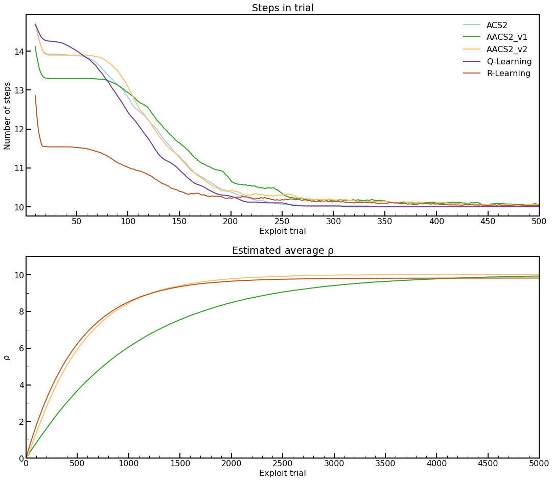
Fig. 5.3 Performance in FSW-10 environment. Plots are averaged over 50 experiments. A moving average with window 25 was applied for the number of steps. Notice that the abscissa on both plots is scaled differently.
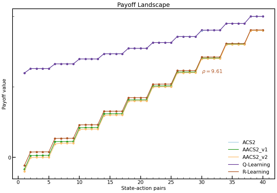
Fig. 5.4 Payoff Landscape for the FSW-10 environment. Payoff values were obtained after 10000 trials. For the Q-Learning and R-Learning, the same learning parameters were applied.
Statistical verification
To statistically assess the population size, the posterior data distribution was modelled using 50 metric values collected in the last trial and then sampled with 100,000 draws.
def build_models(dfs: Dict[str, pd.DataFrame], field: str, query_condition: str):
    results = {}

    for name, df in dfs.items():
        data_arr = df.query(query_condition)[field].to_numpy()
        bayes_model = bayes_estimate(data_arr)
        results[name] = (bayes_model['mu'], bayes_model['std'])

    return results


experiments_data = {
    'fsw10_acs2': fsw10_acs2_metrics.query('agent == "ACS2"'),
    'fsw10_aacs2v1': fsw10_acs2_metrics.query('agent == "AACS2_v1"'),
    'fsw10_aacs2v2': fsw10_acs2_metrics.query('agent == "AACS2_v2"'),
    'fsw10_qlearning': pd.DataFrame(q_learning_runs[0]),
    'fsw10_rlearning': pd.DataFrame(r_learning_runs[0]),

    'fsw20_acs2': fsw20_acs2_metrics.query('agent == "ACS2"'),
    'fsw20_aacs2v1': fsw20_acs2_metrics.query('agent == "AACS2_v1"'),
    'fsw20_aacs2v2': fsw20_acs2_metrics.query('agent == "AACS2_v2"'),
    'fsw20_qlearning': pd.DataFrame(q_learning_runs[1]),
    'fsw20_rlearning': pd.DataFrame(r_learning_runs[1]),

    'fsw40_acs2': fsw40_acs2_metrics.query('agent == "ACS2"'),
    'fsw40_aacs2v1': fsw40_acs2_metrics.query('agent == "AACS2_v1"'),
    'fsw40_aacs2v2': fsw40_acs2_metrics.query('agent == "AACS2_v2"'),
    'fsw40_qlearning': pd.DataFrame(q_learning_runs[2]),
    'fsw40_rlearning': pd.DataFrame(r_learning_runs[2]),
}

@get_from_cache_or_run(cache_path=f'{cache_dir}/fsw/bayes/steps.dill')
def build_steps_models(dfs: Dict[str, pd.DataFrame]):
    return build_models(dfs, field='steps_in_trial', query_condition=f'trial == {trials - 1}')

@get_from_cache_or_run(cache_path=f'{cache_dir}/fsw/bayes/rho.dill')
def build_rho_models(dfs: Dict[str, pd.DataFrame]):
    filtered_dfs = {}
    for k, v in dfs.items():
        if any(r_model for r_model in ['aacs2v1', 'aacs2v2', 'rlearning'] if k.endswith(r_model)):
            filtered_dfs[k] = v

    return build_models(filtered_dfs, field='rho', query_condition=f'trial == {trials - 1}')

steps_models = build_steps_models(experiments_data)
rho_models = build_rho_models(experiments_data)

def print_bayes_table(name_prefix, steps_models, rho_models):
    print_row = lambda r: f'{round(r[0].mean(), 2)} ± {round(r[0].std(), 2)}'
    rho_data = [print_row(v) for name, v in rho_models.items() if name.startswith(name_prefix)]

    bayes_table_data = [
        ['steps in last trial'] + [print_row(v) for name, v in steps_models.items() if name.startswith(name_prefix)],
        ['average reward per step', '-', rho_data[0], rho_data[1], '-', rho_data[2]]
    ]

    table = tabulate(bayes_table_data,
                     headers=['', 'ACS2', 'AACS2v1', 'AACS2v2', 'Q-Learning', 'R-Learning'],
                     tablefmt="html", stralign='center')
    return HTML(table)

# add glue outputs
glue('51-fsw10-bayes', print_bayes_table('fsw10', steps_models, rho_models), display=False)
glue('51-fsw20-bayes', print_bayes_table('fsw20', steps_models, rho_models), display=False)
glue('51-fsw40-bayes', print_bayes_table('fsw40', steps_models, rho_models), display=False)
ACS2 AACS2v1 AACS2v2 Q-Learning R-Learning steps in last trial 10.0 ± 0.0 10.0 ± 0.0 10.0 ± 0.0 10.0 ± 0.0 10.0 ± 0.0 average reward per step - 9.93 ± 0.01 10.01 ± 0.01 - 9.81 ± 0.0
ACS2 AACS2v1 AACS2v2 Q-Learning R-Learning steps in last trial 20.0 ± 0.0 20.0 ± 0.0 20.0 ± 0.0 20.0 ± 0.0 20.0 ± 0.0 average reward per step - 4.99 ± 0.01 5.0 ± 0.01 - 4.9 ± 0.0
ACS2 AACS2v1 AACS2v2 Q-Learning R-Learning steps in last trial 40.0 ± 0.0 40.0 ± 0.0 40.0 ± 0.0 40.0 ± 0.0 40.0 ± 0.0 average reward per step - 2.51 ± 0.0 2.51 ± 0.01 - 2.45 ± 0.0
Observations
The size of the environment used on Figure 5.3 was chosen to be \(n = 10\), resulting in \(2n + 1 = 21\) distinct states. Statistical inference proves that the undiscounted versions of rewarding manage to properly discriminate between worthwhile states without fluctuations for all problem sizes.
The same Figure depicts that agents can learn in a more challenging environment without problems. It takes about 250 trials to perform an optimal number of steps to reach the reward state. The \(\rho\) parameter converges with the same dynamics as the Corridor environment from the previous section.
The payoff-landscape Figure 5.4 shows that the average value estimate is very close to the one calculated by the R-learning algorithm. The difference is primarily visible in the state-action pairs located afar from the final state. The discounted versions of the algorithms performed precisely the same.